行人重识别
这是近几年挺火的一个的一个课题,大概就是研究不同摄像头之间的人物匹配。如下图:
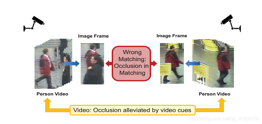
这两个摄像头拍到的两个人,现在我们的任务是检测这两个是否是同一个人。有些思路是在图片上进行处理,但是这样就忽略了人行为的特征,我们这是基于
的数据进行训练。
思路
我们记一个人的特征量
,那么两个人之间的距离就是
。
我们训练的思路是,我们要保证正确答案和错误答案之间隔一个margin。也就是
那么,为了使答案更准确,我们希望下面这个尽量小:
同时,我们也希望下面这个正确距离比较小:
所以我们就得到目标函数
其中,我们距离
用马氏距离表示
现在,为了去简化我们的符号,我们记
那么,距离函数就可以化简为
。
那么,我们的目标函数就是
有了这个式子,我们计算梯度函数:
然后我们利用随机梯度下降算法就可以求解
了。
算法流程
M_0=I;  % 单位矩阵
N(M_0)=[];
G_t=[];
t=0;
while(t<1000 && 不收敛){
	对于每个点,找出来距离最近的点
	对于不满足,两点之间距离隔margin的,放入N(M_t)中
	计算G_t
	M_{t+1} = M_t - \alpha * G_t
	投影M矩阵
}
具体代码实现
现在我们由这几个数据:
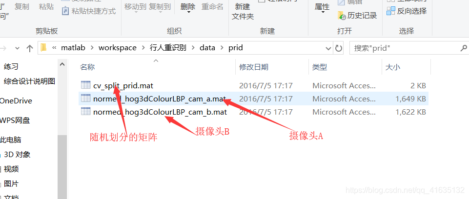
首先,导出数据:
load('cv_split_prid.mat')					%加载随机划分178个数的矩阵
load('normed_hog3dColourLBP_cam_a.mat');	%加载摄像头A的数据
cam1_feature=double(X');
load('normed_hog3dColourLBP_cam_b.mat');  %加载摄像头B的数据
cam2_feature=double(X');
cam1_count=ones(1,178);					%记录  对于摄像头A,每个人多少组数据
cam2_count=ones(1,178);					%记录  对于摄像头B,每个人多少组数据
pars.dem_pca = 177;						%PCA降维到177
然后为了后面的方便,我们将每个人的数据分开。
cam1_feat=feature_mat2cell(cam1_feature,cam1_count);		%摄像头A每个人的cell数据集
cam2_feat=feature_mat2cell(cam2_feature,cam2_count);		%摄像头B每个人的cell数据集
其中feature_mat2cell函数是这样定义的:
function feature_cell=feature_mat2cell(feature_mat,count)
    NumOfPerson = length(count);
    feature_cell=cell(1,NumOfPerson);
    temp_start=1;
    for iPerson=1:NumOfPerson
        num_count=count(iPerson);
        temp_end=temp_start+num_count-1;
        feature_cell{iPerson}=zeros(size(feature_mat,1),num_count);
        feature_cell{iPerson}=feature_mat(:,temp_start:temp_end);
        temp_start=temp_end+1;
    end
end
第三步,拆分数据。我们将数据拆分为两部分,训练集和测试集。
训练集记做:
测试集的测试数据:
。
测试集的答案数据:
。
其中,分别对应的度数列,也就是每一组数据对应多少个数据为:
、
和
。
[TrainingTargetDataSetC,GalleryDataSetC,TestingTargetDataSetC,CountOfTrainingTargetSamples,CountOfGalleryTargetSamples,CountOfTestingTargetSamples]= spilt_dataset(cam1_feat,cam2_feat,target);
其中, 代表的是一组打乱之后的数据,是这样处理的
for s = 1:10
    target = ls_set(s,:);			% 在这个文件中 cv_split_prid.mat
    % 这里省略下面的主体函数
end
其中spilt_dataset函数是这样定义的:
function [xtr,xg,xt,ctr,cg,ct]= spilt_dataset(cam1_feat,cam2_feat,target)
    %% 输出解释:
    % xtr-训练集的数据,
    % xg--镜头A的后半部分,
    % xt--镜头B的后半部分,
    % ctr--训练集的个数列
    % cg--镜头A的后半部分个数列
    % ct--镜头B的后半部分个数列
    %% 输入解释:
    %cam1_feat,cam2_feat: 镜头A,B的每个人的cell
    %target : 排序之后每个人的标签

    %% 分割数据集
    threshold = 10;                             % 每个集合中每个人的【最大】样本值
    shot_flag=1;                                % 单镜头设置1,多镜头设置0

    NumOfPerson=size(target,2);
    NumOfTraining=fix(NumOfPerson/2);
    NumOfGallery= NumOfPerson - NumOfTraining;
    TrainingTarget = target(1:NumOfTraining);

    xtr=[];
    xg=[];
    xt=[];
    ctr=[];
    cg=[];
    ct=[];
    %% 获得训练集
     for i=1:NumOfTraining  %遍历前半部分
         current_Training_featC=[cam1_feat{TrainingTarget(i)} cam2_feat{TrainingTarget(i)}]; % 将摄像头A和摄像头B的数据,水平排开
         current_Training_count=size(current_Training_featC,2);             %获取个数
         if   current_Training_count > threshold                  % 如果大于最大值
            target_temp = randperm(current_Training_count);       % 随机数
            xtr =[xtr current_Training_featC(:,target_temp(1:threshold))]; % xtr并上前threshold个
            ctr =[ctr threshold];                                 % ctr 并上个数
         else
            xtr =[xtr current_Training_featC];                    % xtr并上current_Training_featC
            ctr =[ctr current_Training_count];                   % ctr并上个数
         end
     end

     %% 用来检测答案的后半部分训练集的镜头A
     for i=1:NumOfGallery        %遍历后半部分
         cam1RemainDataSetC=cam1_feat;
         cam1RemainDataSetC(:,TrainingTarget)=[];       %将已经被选在训练集的元素清空
         current_Gallery_featC=cam1RemainDataSetC{i};
         current_Gallery_count=size(current_Gallery_featC,2); %获取每个人元素的个数
         target_temp = randperm(current_Gallery_count);
         if shot_flag                        % 如果是单镜头
             xg= [xg current_Gallery_featC(:, target_temp(1))];
             cg = ones(1,NumOfGallery);
         else                                % 如果是多镜头,选取最多不超过十个
            if  current_Gallery_count > threshold
                target_temp = randperm(current_Gallery_count);
                xg=[xg current_Gallery_featC(:,target_temp(1:threshold))];
                cg =[cg threshold];
            else
                xg =[xg current_Gallery_featC];
                cg =[ cg current_Gallery_count];
            end
         end
     end
     %% 获得测试集,用来检测答案的后半部分训练集的镜头B,也就是答案
     for i=1:NumOfGallery
         cam2RemainDataSetC=cam2_feat;
         cam2RemainDataSetC(:,TrainingTarget)=[];
         current_Testing_featC=cam2RemainDataSetC{i};
         current_Testing_count=size(current_Testing_featC,2);
         if   current_Testing_count > threshold
            target_temp = randperm(current_Testing_count);
             xt =[ xt current_Testing_featC(:,target_temp(1:threshold))];
             ct =[ct threshold];
         else
             xt =[ xt current_Testing_featC];
             ct =[ ct current_Testing_count];
         end
     end
end
很明显,他们这是利用
中已经划分好的数据顺序,对数据进行划分。
差不多这样的划分,相邻的两个为一个训练
。
就是A摄像头剩下的部分,
是B摄像头剩下的部分。当然,他们的顺序都是互相对应的。
第四步,
降维,因为数据的维度是
,维度太高了,不利于进行训练。这个好像利用了
数据降维。现在没太多时间看,反正就是降维成[177,178],代码如下,到时候再好好研究。
function [coeff, score, latent, tsquare] = princompLX(X,econFlag)
    %% 功能介绍
    % 主成分分析函数
    %数据矩阵X,并返回主成分系数,也称为载荷。
    %行X代表观测值,列X代表变量。
    %coeff是一个p×p矩阵,每一列包含一个主成分的系数。这些列按减少分量方差的顺序排列。
    %princompLX通过从列中减去来对X进行中心化,但不对X的列进行缩放。,基于相关性,使用PRINCOMCountOfDim(ZSCORE(X))。
    %要在协方差或相关矩阵上直接执行主成分分析,请使用PCACOV。[COEFF, SCORE] = PRINCOMP(X)返回主成分得分,即,即X在主分量空间中的表示形式。分数的行对应观察值,列对应组件。[COEFF, SCORE, potential] = PRINCOMP(X)返回主成分方差,即的特征值。
    %[COEFF, SCORE, potential, TSQUARED] = PRINCOMP(X)返回Hotelling的T-squared统计数据,用于X中的每个观察。
    %当N <= P时,SCORE(:,N:P)和potential (N:P)必然为零,COEFF(:,N:P)的列定义了正交于X的方向。
    %[…= PRINCOMP(X,'econ')只返回不一定为零的潜伏期元素,即,当N <= P时,只有前N-1,以及相应的COEFF和SCORE列。当P >> N时,这个速度会显著加快。参见BARTTEST, BIPLOT, CANONCORR, FACTORAN, PCACOV, PCARES, ROTATEFACTORS。
    %当X的变量多于观察值时,默认行为是返回所有pc的变量,即使是那些方差为零的。当econFlag是“econ”时,这些将不会被返回。
    if nargin < 2,
        econFlag = 0;
    end
    [CountOfNum,CountOfDim] = size(X);
    if isempty(X)           %如果是空的话,直接返回零阵
        CountOfDimOrZero = ~isequal(econFlag, 'econ') * CountOfDim;
        coeff = zeros(CountOfDim,CountOfDimOrZero);
        coeff(1:CountOfDim+1:end) = 1;
        score = zeros(CountOfNum,CountOfDimOrZero);
        latent = zeros(CountOfDimOrZero,1);
        tsquare = zeros(CountOfNum,1);
        return
    end

    X= bsxfun(@minus,X,mean(X,1));          % 标准化
    if nargout < 2
        if CountOfNum >= CountOfDim && (isequal(econFlag,0) || isequal(econFlag,'econ'))
            [coeff,~] = eig(X'*X);
            coeff = fliplr(coeff);
        else
            [~,~,coeff] = svd(X,econFlag);
        end
        % When econFlag is 'econ', only (n-1) components should be returned.
        % See comment below.
        if (CountOfNum <= CountOfDim) && isequal(econFlag, 'econ')
            coeff(:,CountOfNum) = [];
        end
    else
        r = min(CountOfNum-1,CountOfDim); % max possible rank of X

        % The principal component coefficients are the eigenvectors of
        % S = X'*X./(n-1), but computed using SVD.
        [U,sigma,coeff] = svd(X,econFlag); % put in 1rt(n-1) later

        % Project X onto the principal component axes to get the scores.
        if CountOfNum == 1 % sigma might have only 1 row
            sigma = sigma(1);
        else
            sigma = diag(sigma);
        end
        score = bsxfun(@times,U,sigma'); % == X*coeff
        sigma = sigma ./ sqrt(CountOfNum-1);

        % When X has at least as many variables as observations, eigenvalues
        % n:p of S are exactly zero.
        if CountOfNum <= CountOfDim
            % When econFlag is 'econ', nothing corresponding to the zero
            % eigenvalues should be returned.  svd(,'econ') won't have
            % returned anything corresponding to components (n+1):p, so we
            % just have to cut off the n-th component.
            if isequal(econFlag, 'econ')
                sigma(CountOfNum,:) = []; % make sure this shrinks as a column
                coeff(:,CountOfNum) = [];
                score(:,CountOfNum) = [];

            % Otherwise, set those eigenvalues and the corresponding scores to
            % exactly zero.  svd(,0) won't have returned columns of U
            % corresponding to components (n+1):p, need to fill those out.
            else
                sigma(CountOfNum:CountOfDim,1) = 0; % make sure this extends as a column
                score(:,CountOfNum:CountOfDim) = 0;
            end
        end

        % The variances of the pc's are the eigenvalues of S = X'*X./(n-1).
        latent = sigma.^2;

        % Hotelling's T-squared statistic is the sum of squares of the
        % standardized scores, i.e., Mahalanobis distances.  When X appears to
        % have column rank < r, ignore components that are orthogonal to the
        % data.
        if nargout == 4
            if CountOfNum > 1
                q = sum(sigma > max(CountOfNum,CountOfDim).*eps(sigma(1)));
                if q < r
                    warning('stats:princomp:colRankDefX', ...
                            ['Columns of X are linearly dependent to within machine precision.\n' ...
                             'Using only the first %d components to compute TSQUARED.'],q);
                end
            else
                q = 0;
            end
            tsquare = (CountOfNum-1) .* sum(U(:,1:q).^2,2); % == sum((score*diag(1./sigma)).^2,2)
        end
    end
end
第五步,正文开始。
因为我们的目标是使
这个函数尽量小,我们的工作就是先求
和
。函数如下:
function [PosDiffSetC,NegDiffSetC,PosAmountEachClass,NegAmountEachClass,PosDiffIdC,NegDiffIdC,PosClassDiffIdC,NegClassDiffIdC] = MakePosNegSubsetExt(DataSetC,CountOfSampleEachClass,IsAbs,GroupPointAmount)
%% 输入介绍
% CountOfSampleEachClass = 获取每个人的数据数,这个例子为[2,2,,,,2],A一个B一个
% DataSetC 训练集,先在数据集已经提取主成分由[n,178] => [177,178]
% GroupPointAmount 这是啥?先不管了
% IsAbs 取绝对值
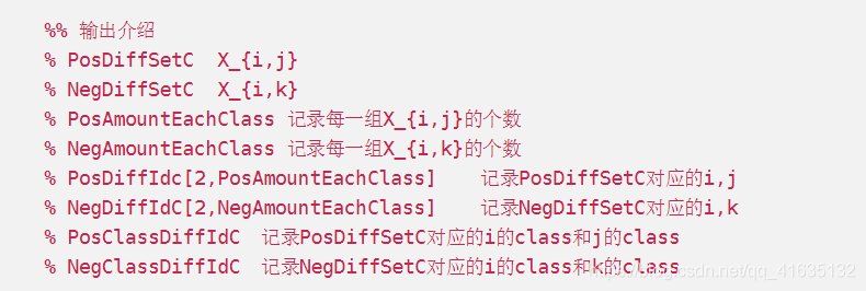
%% 输出介绍
% PosDiffSetC X_{i,j}
% NegDiffSetC X_{i,k}
% PosAmountEachClass 记录每一组X_{i,j}的个数
% NegAmountEachClass 记录每一组X_{i,k}的个数
% PosDiffIdc[2,PosAmountEachClass] 记录PosDiffSetC对应的i,j
% NegDiffIdC[2,NegAmountEachClass] 记录NegDiffSetC对应的i,k
% PosClassDiffIdC 记录PosDiffSetC对应的i的class和j的class
% NegClassDiffIdC 记录NegDiffSetC对应的i的class和k的class
%% 获取基本信息
ClassCount = length(CountOfSampleEachClass); % 训练集组数
SampleCount = sum(CountOfSampleEachClass); % 数据组数
Dim_NewData = round(size(DataSetC,1) / GroupPointAmount); % 训练集的列
Dim_OriData = size(DataSetC,1); % 训练集的列
%% 返回变量
IntraDiffCount = sum(CountOfSampleEachClass .* (CountOfSampleEachClass - 1));
PosDiffSetC = zeros(Dim_NewData,IntraDiffCount);
PosAmountEachClass = zeros(1,sum(CountOfSampleEachClass));
PosDiffIdC = zeros(2,IntraDiffCount);
PosClassDiffIdC = zeros(2,IntraDiffCount);
InterDiffCount = sum(CountOfSampleEachClass .* (SampleCount - CountOfSampleEachClass));
NegDiffSetC = zeros(Dim_NewData,InterDiffCount);
NegAmountEachClass = zeros(1,sum(CountOfSampleEachClass));
NegDiffIdC = zeros(2,InterDiffCount);
NegClassDiffIdC = zeros(2,InterDiffCount);
[ExtentionArrayWithClassLabel] = ... 获取下标数组
StandardExtendClassLableArray(CountOfSampleEachClass);
startpoint_pos = 0;
startpoint_neg = 0;
endpoint_pos = 0;
endpoint_neg = 0;
startpoint = 0;
endpoint = 0;
intra_pair_id = 0;
CumCountOfSampleEachClass = [0 cumsum(CountOfSampleEachClass)]; %
CumCountOfSampleEachClass(end) = [];
DataIndexArray = 1 : SampleCount; % [1,2,3,,,178]
for class_id = 1 : ClassCount % 遍历所有的训练集组
startpoint = endpoint + 1;
endpoint = endpoint + CountOfSampleEachClass(class_id);
CurrentClassDataSetC = DataSetC(:,startpoint : endpoint); %将当前的训练集提取出来
RestClassDataSetC = DataSetC;
RestClassDataSetC(:,startpoint : endpoint) = []; %将提取出来的置为空值
RestDataIndexArray = DataIndexArray;
RestDataIndexArray(startpoint : endpoint) = []; %将提取出来列的下标置为空值
RestExtentionArrayWithClassLabel = ExtentionArrayWithClassLabel;
RestExtentionArrayWithClassLabel(startpoint : endpoint) = []; %将这个也设为空
RestClassSampleAmount = size(RestClassDataSetC,2); % 178-2=176
OrderRecorrectArray = ones(CountOfSampleEachClass(class_id),1); %[2,1]
for sample_id = 1 : CountOfSampleEachClass(class_id) % 遍历每一组的所有数据
intra_pair_id = intra_pair_id + 1;
rest_inner_class = CountOfSampleEachClass(class_id) - 1; % start与end的跨度,自然就是Count-1
startpoint_pos = endpoint_pos + 1;
endpoint_pos = endpoint_pos + rest_inner_class;
startpoint_neg = endpoint_neg + 1;
endpoint_neg = endpoint_neg + RestClassSampleAmount;
current_vector = CurrentClassDataSetC(:,sample_id); % 提取当前数据向量
% get intra class diff vectors
TempCurrentClassDataSetC = CurrentClassDataSetC;
TempCurrentClassDataSetC(:,sample_id) = []; % 将当前数据的当前向量提取出来
DiffDataSetC = ...
current_vector * ones(1,rest_inner_class) ... 将当前行铺开成TempCurrentClassDataSetC大小
- TempCurrentClassDataSetC; % 相减
CurrentOrderRecorrectArray = OrderRecorrectArray;
CurrentOrderRecorrectArray(sample_id) = [];
DiffDataSetC = DiffDataSetC * diag(CurrentOrderRecorrectArray); %将所有(差异)加起来
OrderRecorrectArray(sample_id) = -1; % 用过了,置为-1
if IsAbs == 1
DiffDataSetC = abs(DiffDataSetC);
end
if GroupPointAmount > 1
startpoint_group = 0;
endpoint_group = 0;
sub_dim = 0;
while 1
startpoint_group = endpoint_group + 1;
endpoint_group = endpoint_group + GroupPointAmount;
if endpoint_group > Dim_OriData
endpoint_group = Dim_OriData;
end
sub_dim = sub_dim + 1;
PosDiffSetC(sub_dim,startpoint_pos : endpoint_pos) = ...
sum(DiffDataSetC(startpoint_group : endpoint_group,:));
if endpoint_group == Dim_OriData
break;
end
end
else
PosDiffSetC(:,startpoint_pos : endpoint_pos) = DiffDataSetC;
end
PosAmountEachClass(intra_pair_id) = size(DiffDataSetC,2);
PosDiffIdC(1,startpoint_pos : endpoint_pos) ...
= CumCountOfSampleEachClass(class_id) + sample_id;
TempArray = 1 : CountOfSampleEachClass(class_id);
TempArray(sample_id) = [];
PosDiffIdC(2,startpoint_pos : endpoint_pos) ...
= CumCountOfSampleEachClass(class_id) + TempArray;
PosClassDiffIdC(1,startpoint_pos : endpoint_pos) = class_id;
PosClassDiffIdC(2,startpoint_pos : endpoint_pos) = class_id;
% get inter class diff vectors
DiffDataSetC = ...
current_vector * ones(1,RestClassSampleAmount) ...
- RestClassDataSetC;
if IsAbs == 1
DiffDataSetC = abs(DiffDataSetC);
end
if GroupPointAmount > 1
startpoint_group = 0;
endpoint_group = 0;
sub_dim = 0;
while 1
startpoint_group = endpoint_group + 1;
endpoint_group = endpoint_group + GroupPointAmount;
if endpoint_group > Dim_OriData
endpoint_group = Dim_OriData;
end
sub_dim = sub_dim + 1;
NegDiffSetC(sub_dim,startpoint_neg : endpoint_neg) = ...
sum(DiffDataSetC(startpoint_group : endpoint_group,:));
if endpoint_group == Dim_OriData
break;
end
end
else
NegDiffSetC(:,startpoint_neg : endpoint_neg) = DiffDataSetC;
end
NegDiffIdC(1,startpoint_neg : endpoint_neg) = ...
CumCountOfSampleEachClass(class_id) + sample_id;
NegDiffIdC(2,startpoint_neg : endpoint_neg) = ...
RestDataIndexArray;
NegClassDiffIdC(1,startpoint_neg : endpoint_neg) = class_id;
NegClassDiffIdC(2,startpoint_neg : endpoint_neg) = ...
RestExtentionArrayWithClassLabel;
NegAmountEachClass(intra_pair_id) = size(DiffDataSetC,2);
end
end
end
这些变量的介绍都在这里了,应该挺容易理解。
第六步,计算
这个函数是为了计算
,因为经常用到,这里使用了快速写法。
function res=SOD(x,a,b)
    % equivalent to:
    %
    % res=zeros(size(x,1));
    % for i=1:n
    %   res=res+x(:,a(i))*x(:,b(i))';
    % end;
    [D,N]=size(x);
    B=round(2500/D^2*1000000);
    res=zeros(D^2,1);
    for i=1:B:length(a)
      BB=min(B,length(a)-i);
      Xa=x(:,a(i:i+BB));
      Xb=x(:,b(i:i+BB));
      XaXb=Xa*Xb';
      res=res+vec(Xa*Xa'+Xb*Xb'-XaXb-XaXb');
      if(i>1)   fprintf('.');end;
    end;
    res=mat(res);
end
function M=mat(C)
    r=round(sqrt(size(C,1)));
    M=reshape(C,r,r);
end
function C=vec(M)
    C=M(:);
end
第七步,计算并更新随机梯度函数
。
function  [PosDiffSetC,NegDiffSetC,PosDiffIdC,NegDiffIdC,df_new,loss]=computeGradient(x,CountOfSampleEachClass,L,S,pars)

N=length(CountOfSampleEachClass);
[PosDiffSetC,NegDiffSetC,PosAmountEachClass,NegAmountEachClass,PosDiffIdC,NegDiffIdC,~] = MakePosNegSubsetExt(x,CountOfSampleEachClass,1,1);

    %找到不匹配的最小的那个
    MDN=zeros(1,size(CountOfSampleEachClass,2));
    mc_start=0;
    mc_end=0;
    NegDiffSubset=cell(1,N);
    trigger=zeros(1,N);
    for c = 1:N
        mc_temp = CountOfSampleEachClass(c)*(S-CountOfSampleEachClass(c));
        mc_start=mc_end+1;
        mc_end=mc_start+mc_temp-1;
        NegDiffSubset{c}=NegDiffSetC(:,mc_start:mc_end);
        [MDN(:,c),trigger_c]= min(sum((L*NegDiffSubset{c}).^2,1));
        trigger(1,c)= mc_start + trigger_c-1;
        mc_temp=0;
    end
    %找到最小的编号
    TriNegDiffIdC=NegDiffIdC(:,trigger);

    % 计算匹配的距离
    c=0;
    nc_start=0;
    nc_end=0;
    PosDiffSubset=cell(1,N);
    notrigger = [];
    loss=zeros(1,c);
    for c = 1:N
        nc_temp = CountOfSampleEachClass(c)*(CountOfSampleEachClass(c)-1)/2;
        nc_start=nc_end+1;
        nc_end=nc_start+nc_temp-1;
        PosDiffSubset{c}=PosDiffSetC(:,nc_start:nc_end);
        notrigger_temp = find(sum((L*PosDiffSubset{c}).^2,1) - MDN(:,c) <0) ;
        if sum((L*PosDiffSubset{c}).^2,1) - MDN(:,c) > 0,
            loss(1,c)=sum(sum((L*PosDiffSubset{c}).^2,1) - MDN(:,c));
        else loss(1,c)=0;
        end
        notrigger =[notrigger nc_start+notrigger_temp-1];
        nc_temp=0;
    end
        TriPosDiffIdC=PosDiffIdC;
        TriPosDiffIdC(:,notrigger)=[];
    if(~pars.quiet)fprintf(['size of trigger:%i \n '],size(TriPosDiffIdC,2));end;

    df=vec(SOD(x,TriPosDiffIdC(1,:),TriPosDiffIdC(2,:))-SOD(x,TriNegDiffIdC(1,:),TriNegDiffIdC(2,:)));
    df_new=df;
end
综上,就大功告成了。
最后在检测一下:
    disp('Average accuracy of rank 1 5 10 15 20');
    FinalRankRate=mean(RankRateMat,1);      %求平均值
    disp(FinalRankRate([1 5 10 15 20]));
    plot(FinalRankRate,'b-v');