xgboost原理及python实现

xgboost原理

xgboost的python实现(Aarshay Jain的文章)

1. The XGBoost Advantage

2. XGBoost Parameters

General Parameters

Booster Parameters

Learning Task Parameters

3. Parameter Tuning with Example

General Approach for Parameter Tuning

Step 1: Fix learning rate and number of estimators for tuning tree-based parameters

Step 2: Tune max_depth and min_child_weight

Step 3: Tune gamma

Step 4: Tune subsample and colsample_bytree

Step 5: Tuning Regularization Parameters

Step 6: Reducing Learning Rate

End Notes

xgboost原理

具体了解还是要看Tianqi Chen大佬文章

决策树分为分类树和回归树(CART)组成。这里有一个简单的的例子，用来区分人们是否会喜欢电脑游戏。

但是有时候一棵树并不够给力,那么一般会加上bagging的算法或者加上boosting的算法使得树模型更加有力.可以尝试对每棵树的预测得分进行求和，得到最终的得分。如下图所示，一个重要的事实是这两棵树试图互补。数学上表示为

那么对于该树加上正则化以及一些树的复杂度的约束后可以将目标函数写成

当用bagging的简单算法后,可以将每棵树以一定的权重进行投票,这个比较简单,当用boosting的算法,boosting的思路大致如下

当用了boosting的算法之后,我们将上式添加正则化项

以及使用平方损失函数,并且将常数项移出,利用泰勒公式进行近似约等,其中g为一阶导,h为二阶导

将树的正则化项加入到公式中,其中将数据分为两个积分符号的形式(一个为树的叶子,一个为每个叶子上的数据),并且将小写的g和h积分简单写成大写G与H进行进一步化简

对将上式目标函数对w求导求得最优化的obj(带参数的方程用导数求最佳解)

那么我们通过对不同树的目标函数进行上式的对比就行,但是!,不可能将所有的树的模型都知道,所以一般以树生成方法进行判断,每一次生成树时我们将所的的增益通过下式算出来,以此来判断是否要继续生成新的节点

xgboost的python实现(Aarshay Jain的文章)

Aarshay Jain的文章:https://www.analyticsvidhya.com/blog/2016/03/complete-guide-parameter-tuning-xgboost-with-codes-python/

1. The XGBoost Advantage

I’ve always admired the boosting capabilities that this algorithm infuses in a predictive model. When I explored more about its performance and science behind its high accuracy, I discovered many advantages:

Regularization:
- Standard GBM implementation has no regularization like XGBoost, therefore it also helps to reduce overfitting.
- In fact, XGBoost is also known as ‘regularized boosting‘ technique.
Parallel Processing:
- XGBoost implements parallel processing and is blazingly faster as compared to GBM.
- But hang on, we know that boosting is sequential process so how can it be parallelized? We know that each tree can be built only after the previous one, so what stops us from making a tree using all cores? I hope you get where I’m coming from. Check this link out to explore further.
- XGBoost also supports implementation on Hadoop.
High Flexibility
- XGBoost allow users to define custom optimization objectives and evaluation criteria.
- This adds a whole new dimension to the model and there is no limit to what we can do.
Handling Missing Values
- XGBoost has an in-built routine to handle missing values.
- User is required to supply a different value than other observations and pass that as a parameter. XGBoost tries different things as it encounters a missing value on each node and learns which path to take for missing values in future.
Tree Pruning:
- A GBM would stop splitting a node when it encounters a negative loss in the split. Thus it is more of a greedy algorithm.
- XGBoost on the other hand make splits upto the max_depth specified and then start pruning the tree backwards and remove splits beyond which there is no positive gain.
- Another advantage is that sometimes a split of negative loss say -2 may be followed by a split of positive loss +10. GBM would stop as it encounters -2. But XGBoost will go deeper and it will see a combined effect of +8 of the split and keep both.
Built-in Cross-Validation
- XGBoost allows user to run a cross-validation at each iteration of the boosting process and thus it is easy to get the exact optimum number of boosting iterations in a single run.
- This is unlike GBM where we have to run a grid-search and only a limited values can be tested.
Continue on Existing Model
- User can start training an XGBoost model from its last iteration of previous run. This can be of significant advantage in certain specific applications.
- GBM implementation of sklearn also has this feature so they are even on this point.

I hope now you understand the sheer power XGBoost algorithm. Note that these are the points which I could muster. You know a few more? Feel free to drop a comment below and I will update the list.

Did I whet your appetite ? Good. You can refer to following web-pages for a deeper understanding:

2. XGBoost Parameters

The overall parameters have been divided into 3 categories by XGBoost authors:

General Parameters: Guide the overall functioning
Booster Parameters: Guide the individual booster (tree/regression) at each step
Learning Task Parameters: Guide the optimization performed

I will give analogies to GBM here and highly recommend to read this article to learn from the very basics.

General Parameters

These define the overall functionality of XGBoost.

booster [default=gbtree]
- Select the type of model to run at each iteration. It has 2 options:
  - gbtree: tree-based models
  - gblinear: linear models
silent [default=0]:
- Silent mode is activated is set to 1, i.e. no running messages will be printed.
- It’s generally good to keep it 0 as the messages might help in understanding the model.
nthread [default to maximum number of threads available if not set]
- This is used for parallel processing and number of cores in the system should be entered
- If you wish to run on all cores, value should not be entered and algorithm will detect automatically

There are 2 more parameters which are set automatically by XGBoost and you need not worry about them. Lets move on to Booster parameters.

Booster Parameters

Though there are 2 types of boosters, I’ll consider only tree booster here because it always outperforms the linear booster and thus the later is rarely used.

eta [default=0.3]
- Analogous to learning rate in GBM
- Makes the model more robust by shrinking the weights on each step
- Typical final values to be used: 0.01-0.2
min_child_weight [default=1]
- Defines the minimum sum of weights of all observations required in a child.
- This is similar to min_child_leaf in GBM but not exactly. This refers to min “sum of weights” of observations while GBM has min “number of observations”.
- Used to control over-fitting. Higher values prevent a model from learning relations which might be highly specific to the particular sample selected for a tree.
- Too high values can lead to under-fitting hence, it should be tuned using CV.
max_depth [default=6]
- The maximum depth of a tree, same as GBM.
- Used to control over-fitting as higher depth will allow model to learn relations very specific to a particular sample.
- Should be tuned using CV.
- Typical values: 3-10
max_leaf_nodes
- The maximum number of terminal nodes or leaves in a tree.
- Can be defined in place of max_depth. Since binary trees are created, a depth of ‘n’ would produce a maximum of 2^n leaves.
- If this is defined, GBM will ignore max_depth.
gamma [default=0]
- A node is split only when the resulting split gives a positive reduction in the loss function. Gamma specifies the minimum loss reduction required to make a split.
- Makes the algorithm conservative. The values can vary depending on the loss function and should be tuned.
max_delta_step [default=0]
- In maximum delta step we allow each tree’s weight estimation to be. If the value is set to 0, it means there is no constraint. If it is set to a positive value, it can help making the update step more conservative.
- Usually this parameter is not needed, but it might help in logistic regression when class is extremely imbalanced.
- This is generally not used but you can explore further if you wish.
subsample [default=1]
- Same as the subsample of GBM. Denotes the fraction of observations to be randomly samples for each tree.
- Lower values make the algorithm more conservative and prevents overfitting but too small values might lead to under-fitting.
- Typical values: 0.5-1
colsample_bytree [default=1]
- Similar to max_features in GBM. Denotes the fraction of columns to be randomly samples for each tree.
- Typical values: 0.5-1
colsample_bylevel [default=1]
- Denotes the subsample ratio of columns for each split, in each level.
- I don’t use this often because subsample and colsample_bytree will do the job for you. but you can explore further if you feel so.
lambda [default=1]
- L2 regularization term on weights (analogous to Ridge regression)
- This used to handle the regularization part of XGBoost. Though many data scientists don’t use it often, it should be explored to reduce overfitting.
alpha [default=0]
- L1 regularization term on weight (analogous to Lasso regression)
- Can be used in case of very high dimensionality so that the algorithm runs faster when implemented
scale_pos_weight [default=1]
- A value greater than 0 should be used in case of high class imbalance as it helps in faster convergence.

Learning Task Parameters

These parameters are used to define the optimization objective the metric to be calculated at each step.

objective [default=reg:linear]
- This defines the loss function to be minimized. Mostly used values are:
  - binary:logistic –logistic regression for binary classification, returns predicted probability (not class)
  - multi:softmax –multiclass classification using the softmax objective, returns predicted class (not probabilities)
    - you also need to set an additional num_class (number of classes) parameter defining the number of unique classes
  - multi:softprob –same as softmax, but returns predicted probability of each data point belonging to each class.
eval_metric [ default according to objective ]
- The metric to be used for validation data.
- The default values are rmse for regression and error for classification.
- Typical values are:
  - rmse – root mean square error
  - mae – mean absolute error
  - logloss – negative log-likelihood
  - error – Binary classification error rate (0.5 threshold)
  - merror – Multiclass classification error rate
  - mlogloss – Multiclass logloss
  - auc: Area under the curve
seed [default=0]
- The random number seed.
- Can be used for generating reproducible results and also for parameter tuning.

If you’ve been using Scikit-Learn till now, these parameter names might not look familiar. A good news is that xgboost module in python has an sklearn wrapper called XGBClassifier. It uses sklearn style naming convention. The parameters names which will change are:

eta –> learning_rate
lambda –> reg_lambda
alpha –> reg_alpha

You must be wondering that we have defined everything except something similar to the “n_estimators” parameter in GBM. Well this exists as a parameter in XGBClassifier. However, it has to be passed as “num_boosting_rounds” while calling the fit function in the standard xgboost implementation.

I recommend you to go through the following parts of xgboost guide to better understand the parameters and codes:

3. Parameter Tuning with Example

We will take the data set from Data Hackathon 3.x AV hackathon, same as that taken in the GBM article. The details of the problem can be found on the competition page. You can download the data set from here. I have performed the following steps:

City variable dropped because of too many categories
DOB converted to Age | DOB dropped
EMI_Loan_Submitted_Missing created which is 1 if EMI_Loan_Submitted was missing else 0 | Original variable EMI_Loan_Submitted dropped
EmployerName dropped because of too many categories
Existing_EMI imputed with 0 (median) since only 111 values were missing
Interest_Rate_Missing created which is 1 if Interest_Rate was missing else 0 | Original variable Interest_Rate dropped
Lead_Creation_Date dropped because made little intuitive impact on outcome
Loan_Amount_Applied, Loan_Tenure_Applied imputed with median values
Loan_Amount_Submitted_Missing created which is 1 if Loan_Amount_Submitted was missing else 0 | Original variable Loan_Amount_Submitted dropped
Loan_Tenure_Submitted_Missing created which is 1 if Loan_Tenure_Submitted was missing else 0 | Original variable Loan_Tenure_Submitted dropped
LoggedIn, Salary_Account dropped
Processing_Fee_Missing created which is 1 if Processing_Fee was missing else 0 | Original variable Processing_Fee dropped
Source – top 2 kept as is and all others combined into different category
Numerical and One-Hot-Coding performed

For those who have the original data from competition, you can check out these steps from the data_preparation iPython notebook in the repository.

Lets start by importing the required libraries and loading the data:

#Import libraries:
import pandas as pd
import numpy as np
import xgboost as xgb
from xgboost.sklearn import XGBClassifier
from sklearn import cross_validation, metrics   #Additional scklearn functions
from sklearn.grid_search import GridSearchCV   #Perforing grid search

import matplotlib.pylab as plt
%matplotlib inline
from matplotlib.pylab import rcParams
rcParams['figure.figsize'] = 12, 4

train = pd.read_csv('train_modified.csv')
target = 'Disbursed'
IDcol = 'ID'

Note that I have imported 2 forms of XGBoost:

xgb – this is the direct xgboost library. I will use a specific function “cv” from this library
XGBClassifier – this is an sklearn wrapper for XGBoost. This allows us to use sklearn’s Grid Search with parallel processing in the same way we did for GBM

Before proceeding further, lets define a function which will help us create XGBoost models and perform cross-validation. The best part is that you can take this function as it is and use it later for your own models.

def modelfit(alg, dtrain, predictors,useTrainCV=True, cv_folds=5, early_stopping_rounds=50):
    
    if useTrainCV:
        xgb_param = alg.get_xgb_params()
        xgtrain = xgb.DMatrix(dtrain[predictors].values, label=dtrain[target].values)
        cvresult = xgb.cv(xgb_param, xgtrain, num_boost_round=alg.get_params()['n_estimators'], nfold=cv_folds,
            metrics='auc', early_stopping_rounds=early_stopping_rounds, show_progress=False)
        alg.set_params(n_estimators=cvresult.shape[0])
    
    #Fit the algorithm on the data
    alg.fit(dtrain[predictors], dtrain['Disbursed'],eval_metric='auc')
        
    #Predict training set:
    dtrain_predictions = alg.predict(dtrain[predictors])
    dtrain_predprob = alg.predict_proba(dtrain[predictors])[:,1]
        
    #Print model report:
    print "\nModel Report"
    print "Accuracy : %.4g" % metrics.accuracy_score(dtrain['Disbursed'].values, dtrain_predictions)
    print "AUC Score (Train): %f" % metrics.roc_auc_score(dtrain['Disbursed'], dtrain_predprob)
                    
    feat_imp = pd.Series(alg.booster().get_fscore()).sort_values(ascending=False)
    feat_imp.plot(kind='bar', title='Feature Importances')
    plt.ylabel('Feature Importance Score')

This code is slightly different from what I used for GBM. The focus of this article is to cover the concepts and not coding. Please feel free to drop a note in the comments if you find any challenges in understanding any part of it. Note that xgboost’s sklearn wrapper doesn’t have a “feature_importances” metric but a get_fscore() function which does the same job.

General Approach for Parameter Tuning

We will use an approach similar to that of GBM here. The various steps to be performed are:

Choose a relatively high learning rate. Generally a learning rate of 0.1 works but somewhere between 0.05 to 0.3 should work for different problems. Determine the optimum number of trees for this learning rate. XGBoost has a very useful function called as “cv” which performs cross-validation at each boosting iteration and thus returns the optimum number of trees required.
Tune tree-specific parameters ( max_depth, min_child_weight, gamma, subsample, colsample_bytree) for decided learning rate and number of trees. Note that we can choose different parameters to define a tree and I’ll take up an example here.
Tune regularization parameters (lambda, alpha) for xgboost which can help reduce model complexity and enhance performance.
Lower the learning rate and decide the optimal parameters .

Let us look at a more detailed step by step approach.

Step 1: Fix learning rate and number of estimators for tuning tree-based parameters

In order to decide on boosting parameters, we need to set some initial values of other parameters. Lets take the following values:

max_depth = 5 : This should be between 3-10. I’ve started with 5 but you can choose a different number as well. 4-6 can be good starting points.
min_child_weight = 1 : A smaller value is chosen because it is a highly imbalanced class problem and leaf nodes can have smaller size groups.
gamma = 0 : A smaller value like 0.1-0.2 can also be chosen for starting. This will anyways be tuned later.
subsample, colsample_bytree = 0.8 : This is a commonly used used start value. Typical values range between 0.5-0.9.
scale_pos_weight = 1: Because of high class imbalance.

Please note that all the above are just initial estimates and will be tuned later. Lets take the default learning rate of 0.1 here and check the optimum number of trees using cv function of xgboost. The function defined above will do it for us.

#Choose all predictors except target & IDcols
predictors = [x for x in train.columns if x not in [target, IDcol]]
xgb1 = XGBClassifier(
 learning_rate =0.1,
 n_estimators=1000,
 max_depth=5,
 min_child_weight=1,
 gamma=0,
 subsample=0.8,
 colsample_bytree=0.8,
 objective= 'binary:logistic',
 nthread=4,
 scale_pos_weight=1,
 seed=27)
modelfit(xgb1, train, predictors)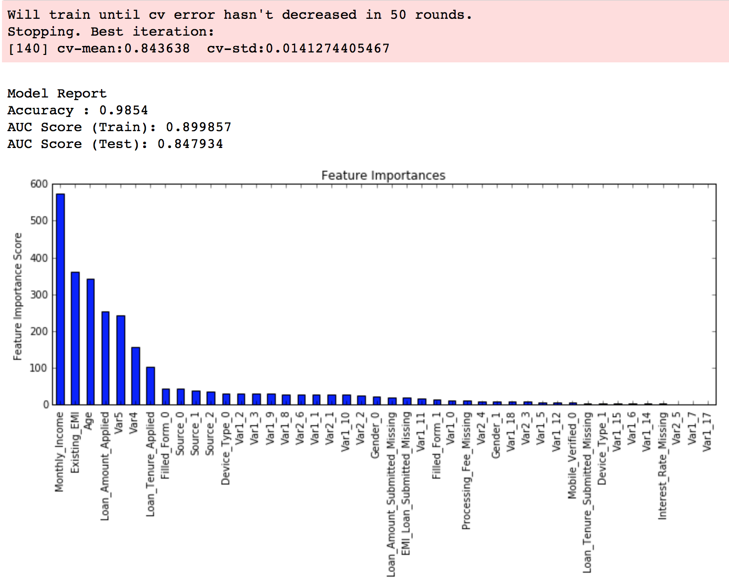

As you can see that here we got 140 as the optimal estimators for 0.1 learning rate. Note that this value might be too high for you depending on the power of your system. In that case you can increase the learning rate and re-run the command to get the reduced number of estimators.

Note: You will see the test AUC as “AUC Score (Test)” in the outputs here. But this would not appear if you try to run the command on your system as the data is not made public. It’s provided here just for reference. The part of the code which generates this output has been removed here.

Step 2: Tune max_depth and min_child_weight

We tune these first as they will have the highest impact on model outcome. To start with, let’s set wider ranges and then we will perform another iteration for smaller ranges.

Important Note: I’ll be doing some heavy-duty grid searched in this section which can take 15-30 mins or even more time to run depending on your system. You can vary the number of values you are testing based on what your system can handle.

param_test1 = {
 'max_depth':range(3,10,2),
 'min_child_weight':range(1,6,2)
}
gsearch1 = GridSearchCV(estimator = XGBClassifier( learning_rate =0.1, n_estimators=140, max_depth=5,
 min_child_weight=1, gamma=0, subsample=0.8, colsample_bytree=0.8,
 objective= 'binary:logistic', nthread=4, scale_pos_weight=1, seed=27), 
 param_grid = param_test1, scoring='roc_auc',n_jobs=4,iid=False, cv=5)
gsearch1.fit(train[predictors],train[target])
gsearch1.grid_scores_, gsearch1.best_params_, gsearch1.best_score_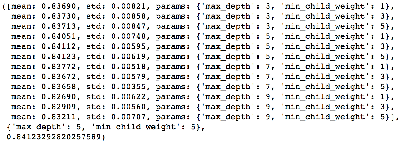

Here, we have run 12 combinations with wider intervals between values. The ideal values are 5 for max_depth and 5 for min_child_weight. Lets go one step deeper and look for optimum values. We’ll search for values 1 above and below the optimum values because we took an interval of two.

param_test2 = {
 'max_depth':[4,5,6],
 'min_child_weight':[4,5,6]
}
gsearch2 = GridSearchCV(estimator = XGBClassifier( learning_rate=0.1, n_estimators=140, max_depth=5,
 min_child_weight=2, gamma=0, subsample=0.8, colsample_bytree=0.8,
 objective= 'binary:logistic', nthread=4, scale_pos_weight=1,seed=27), 
 param_grid = param_test2, scoring='roc_auc',n_jobs=4,iid=False, cv=5)
gsearch2.fit(train[predictors],train[target])
gsearch2.grid_scores_, gsearch2.best_params_, gsearch2.best_score_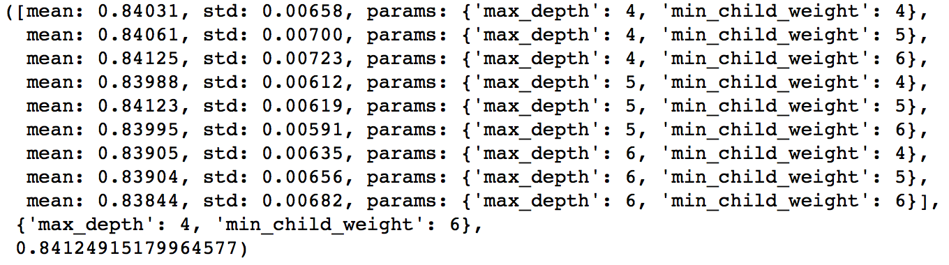

Here, we get the optimum values as 4 for max_depth and 6 for min_child_weight. Also, we can see the CV score increasing slightly. Note that as the model performance increases, it becomes exponentially difficult to achieve even marginal gains in performance. You would have noticed that here we got 6 as optimum value for min_child_weight but we haven’t tried values more than 6. We can do that as follow:.

param_test2b = {
 'min_child_weight':[6,8,10,12]
}
gsearch2b = GridSearchCV(estimator = XGBClassifier( learning_rate=0.1, n_estimators=140, max_depth=4,
 min_child_weight=2, gamma=0, subsample=0.8, colsample_bytree=0.8,
 objective= 'binary:logistic', nthread=4, scale_pos_weight=1,seed=27), 
 param_grid = param_test2b, scoring='roc_auc',n_jobs=4,iid=False, cv=5)
gsearch2b.fit(train[predictors],train[target])

modelfit(gsearch3.best_estimator_, train, predictors)
gsearch2b.grid_scores_, gsearch2b.best_params_, gsearch2b.best_score_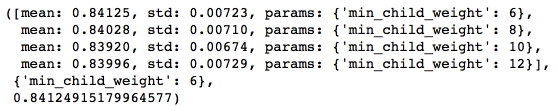

We see 6 as the optimal value.

Step 3: Tune gamma

Now lets tune gamma value using the parameters already tuned above. Gamma can take various values but I’ll check for 5 values here. You can go into more precise values as.

param_test3 = {
 'gamma':[i/10.0 for i in range(0,5)]
}
gsearch3 = GridSearchCV(estimator = XGBClassifier( learning_rate =0.1, n_estimators=140, max_depth=4,
 min_child_weight=6, gamma=0, subsample=0.8, colsample_bytree=0.8,
 objective= 'binary:logistic', nthread=4, scale_pos_weight=1,seed=27), 
 param_grid = param_test3, scoring='roc_auc',n_jobs=4,iid=False, cv=5)
gsearch3.fit(train[predictors],train[target])
gsearch3.grid_scores_, gsearch3.best_params_, gsearch3.best_score_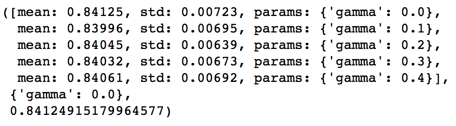

This shows that our original value of gamma, i.e. 0 is the optimum one. Before proceeding, a good idea would be to re-calibrate the number of boosting rounds for the updated parameters.

xgb2 = XGBClassifier(
 learning_rate =0.1,
 n_estimators=1000,
 max_depth=4,
 min_child_weight=6,
 gamma=0,
 subsample=0.8,
 colsample_bytree=0.8,
 objective= 'binary:logistic',
 nthread=4,
 scale_pos_weight=1,
 seed=27)
modelfit(xgb2, train, predictors)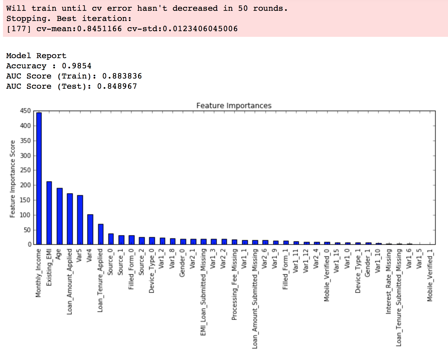

Here, we can see the improvement in score. So the final parameters are:

max_depth: 4
min_child_weight: 6
gamma: 0

Step 4: Tune subsample and colsample_bytree

The next step would be try different subsample and colsample_bytree values. Lets do this in 2 stages as well and take values 0.6,0.7,0.8,0.9 for both to start with.

param_test4 = {
 'subsample':[i/10.0 for i in range(6,10)],
 'colsample_bytree':[i/10.0 for i in range(6,10)]
}
gsearch4 = GridSearchCV(estimator = XGBClassifier( learning_rate =0.1, n_estimators=177, max_depth=4,
 min_child_weight=6, gamma=0, subsample=0.8, colsample_bytree=0.8,
 objective= 'binary:logistic', nthread=4, scale_pos_weight=1,seed=27), 
 param_grid = param_test4, scoring='roc_auc',n_jobs=4,iid=False, cv=5)
gsearch4.fit(train[predictors],train[target])
gsearch4.grid_scores_, gsearch4.best_params_, gsearch4.best_score_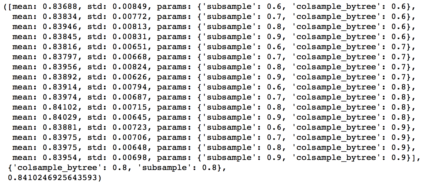

Here, we found 0.8 as the optimum value for both subsample and colsample_bytree. Now we should try values in 0.05 interval around these.

param_test5 = {
 'subsample':[i/100.0 for i in range(75,90,5)],
 'colsample_bytree':[i/100.0 for i in range(75,90,5)]
}
gsearch5 = GridSearchCV(estimator = XGBClassifier( learning_rate =0.1, n_estimators=177, max_depth=4,
 min_child_weight=6, gamma=0, subsample=0.8, colsample_bytree=0.8,
 objective= 'binary:logistic', nthread=4, scale_pos_weight=1,seed=27), 
 param_grid = param_test5, scoring='roc_auc',n_jobs=4,iid=False, cv=5)
gsearch5.fit(train[predictors],train[target])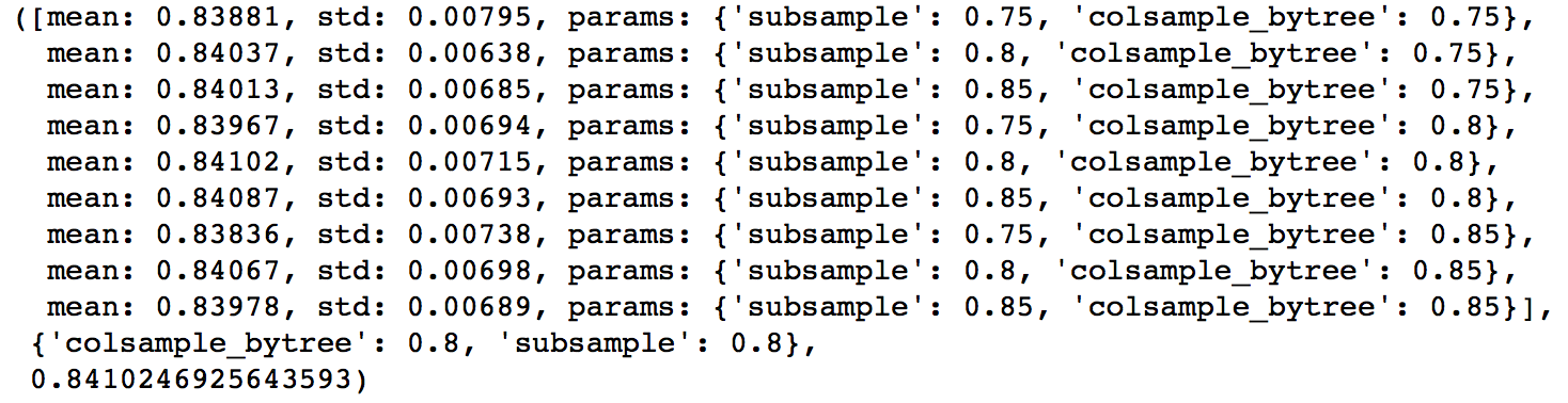

Again we got the same values as before. Thus the optimum values are:

subsample: 0.8
colsample_bytree: 0.8

Step 5: Tuning Regularization Parameters

Next step is to apply regularization to reduce overfitting. Though many people don’t use this parameters much as gamma provides a substantial way of controlling complexity. But we should always try it. I’ll tune ‘reg_alpha’ value here and leave it upto you to try different values of ‘reg_lambda’.

param_test6 = {
 'reg_alpha':[1e-5, 1e-2, 0.1, 1, 100]
}
gsearch6 = GridSearchCV(estimator = XGBClassifier( learning_rate =0.1, n_estimators=177, max_depth=4,
 min_child_weight=6, gamma=0.1, subsample=0.8, colsample_bytree=0.8,
 objective= 'binary:logistic', nthread=4, scale_pos_weight=1,seed=27), 
 param_grid = param_test6, scoring='roc_auc',n_jobs=4,iid=False, cv=5)
gsearch6.fit(train[predictors],train[target])
gsearch6.grid_scores_, gsearch6.best_params_, gsearch6.best_score_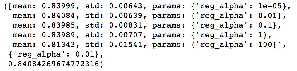

We can see that the CV score is less than the previous case. But the values tried are very widespread, we should try values closer to the optimum here (0.01) to see if we get something better.

param_test7 = {
 'reg_alpha':[0, 0.001, 0.005, 0.01, 0.05]
}
gsearch7 = GridSearchCV(estimator = XGBClassifier( learning_rate =0.1, n_estimators=177, max_depth=4,
 min_child_weight=6, gamma=0.1, subsample=0.8, colsample_bytree=0.8,
 objective= 'binary:logistic', nthread=4, scale_pos_weight=1,seed=27), 
 param_grid = param_test7, scoring='roc_auc',n_jobs=4,iid=False, cv=5)
gsearch7.fit(train[predictors],train[target])
gsearch7.grid_scores_, gsearch7.best_params_, gsearch7.best_score_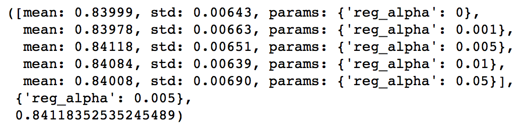

You can see that we got a better CV. Now we can apply this regularization in the model and look at the impact:

xgb3 = XGBClassifier(
 learning_rate =0.1,
 n_estimators=1000,
 max_depth=4,
 min_child_weight=6,
 gamma=0,
 subsample=0.8,
 colsample_bytree=0.8,
 reg_alpha=0.005,
 objective= 'binary:logistic',
 nthread=4,
 scale_pos_weight=1,
 seed=27)
modelfit(xgb3, train, predictors)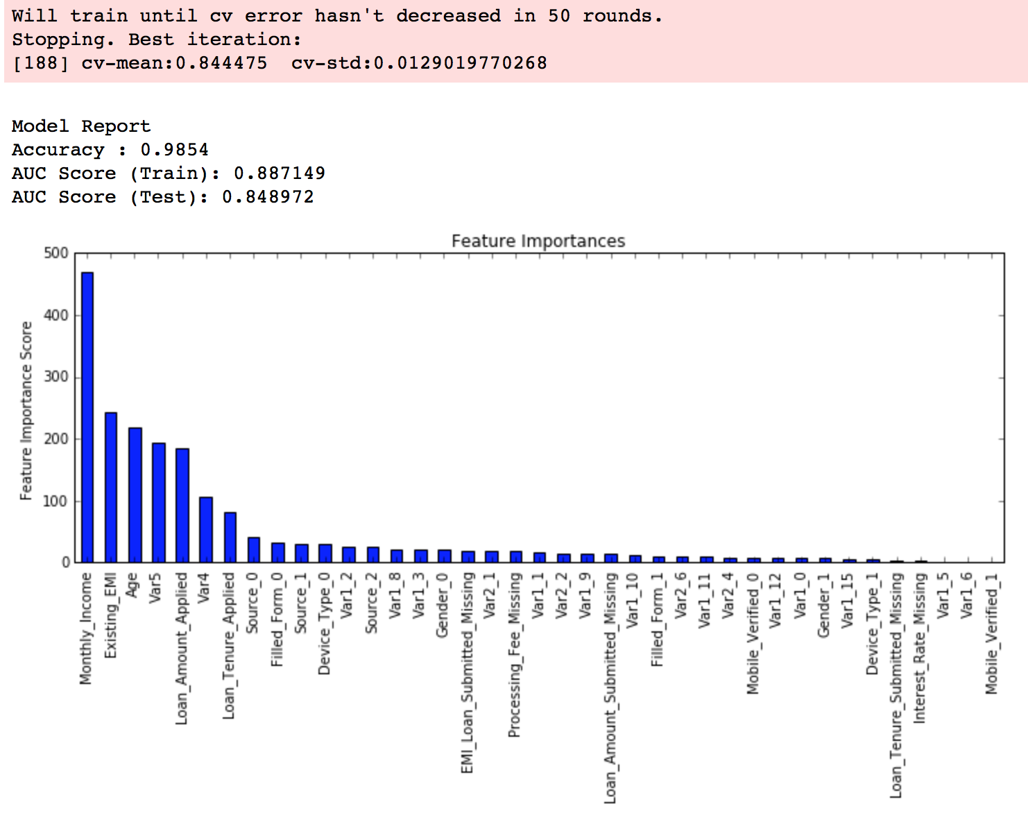

Again we can see slight improvement in the score.

Step 6: Reducing Learning Rate

Lastly, we should lower the learning rate and add more trees. Lets use the cv function of XGBoost to do the job again.

xgb4 = XGBClassifier(
 learning_rate =0.01,
 n_estimators=5000,
 max_depth=4,
 min_child_weight=6,
 gamma=0,
 subsample=0.8,
 colsample_bytree=0.8,
 reg_alpha=0.005,
 objective= 'binary:logistic',
 nthread=4,
 scale_pos_weight=1,
 seed=27)
modelfit(xgb4, train, predictors)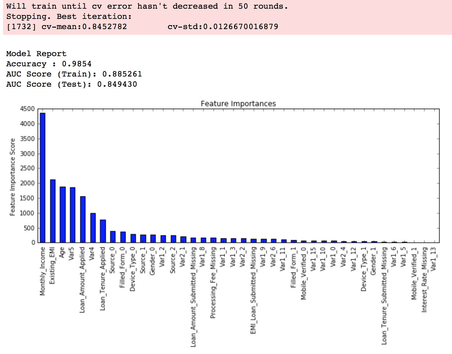

Now we can see a significant boost in performance and the effect of parameter tuning is clearer.

As we come to the end, I would like to share 2 key thoughts:

It is difficult to get a very big leap in performance by just using parameter tuning or slightly better models. The max score for GBM was 0.8487 while XGBoost gave 0.8494. This is a decent improvement but not something very substantial.
A significant jump can be obtained by other methods like feature engineering, creating ensemble of models, stacking, etc

You can also download the iPython notebook with all these model codes from my GitHub account. For codes in R, you can refer to this article.

End Notes

This article was based on developing a XGBoost model end-to-end. We started with discussing why XGBoost has superior performance over GBM which was followed by detailed discussion on the various parameters involved. We also defined a generic function which you can re-use for making models.

Finally, we discussed the general approach towards tackling a problem with XGBoost and also worked out the AV Data Hackathon 3.x problem through that approach.

I hope you found this useful and now you feel more confident to apply XGBoost in solving a data science problem. You can try this out in out upcoming hackathons.

Did you like this article? Would you like to share some other hacks which you implement while making XGBoost models? Please feel free to drop a note in the comments below and I’ll be glad to discuss.