[PyTorch小试牛刀]实战一·使用PyTorch拟合曲线
在深度学习入门的博客中,我们用TensorFlow进行了拟合曲线,到达了不错的效果。
我们现在使用PyTorch进行相同的曲线拟合,进而来比较一下TensorFlow与PyTorch的异同。
搭建神经网络进行训练的步骤基本相同,我们现在开始用PyTorch来实现。
-
问题描述
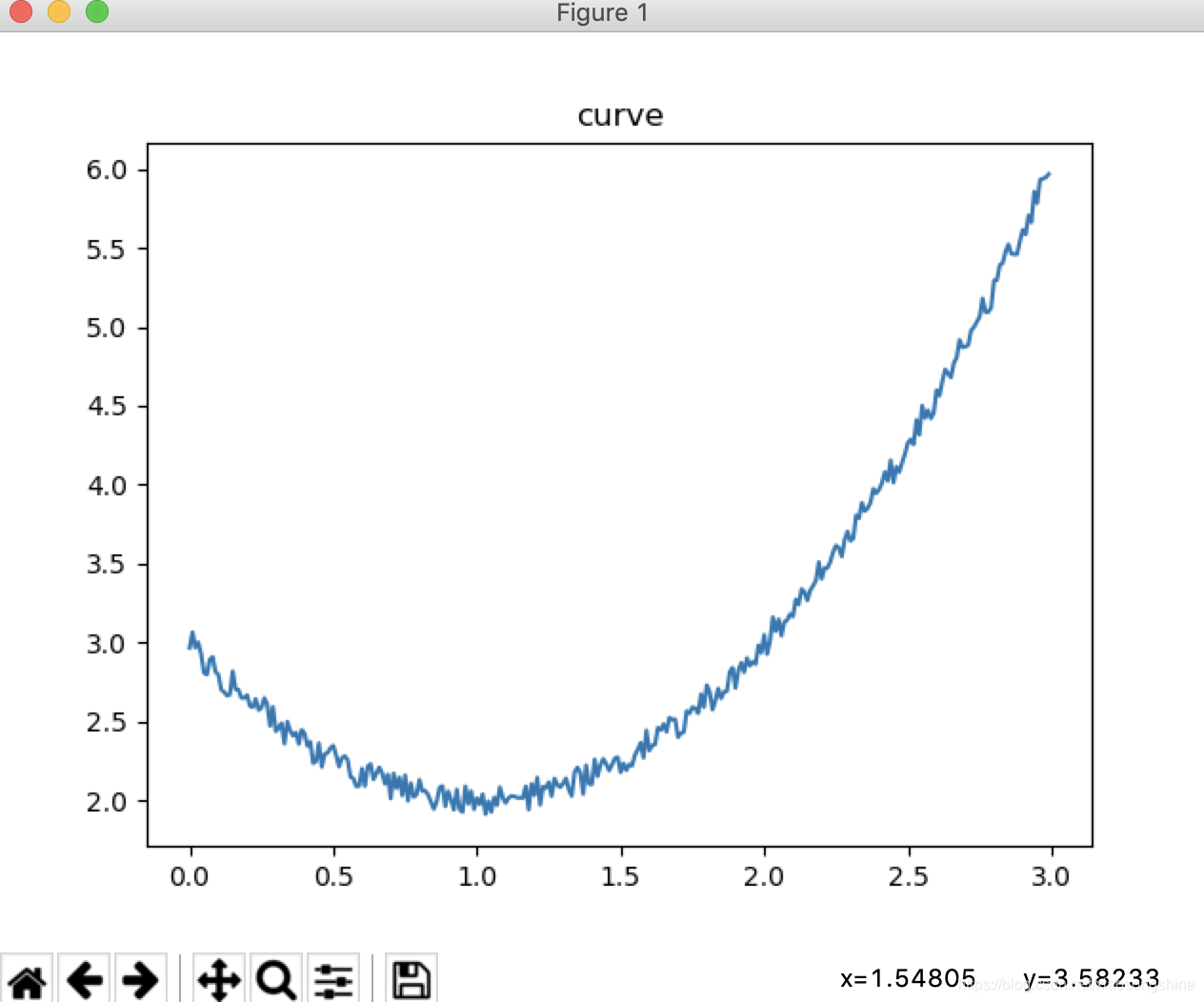
拟合y= x*x -2x +3 + 0.1(-1到1的随机值) 曲线
给定x范围(0,3) -
问题分析
在直线拟合博客中,我们使用最简单的y=wx+b的模型成功拟合了一条直线,现在我们在进一步进行曲线的拟合。简单的y=wx+b模型已经无法满足我们的需求,需要利用更多的神经元来解决问题了。 -
生成数据
import numpy as np
import matplotlib.pyplot as plt
import torch as t
from torch.autograd import Variable as var

def get_data(x,w,b,d):
    c,r = x.shape
    y = (w * x * x + b*x + d)+ (0.1*(2*np.random.rand(c,r)-1))
    return(y)

xs = np.arange(0,3,0.01).reshape(-1,1)
ys = get_data(xs,1,-2,3)

xs = var(t.Tensor(xs))
ys = var(t.Tensor(ys))
生成的数据图像为:
- 搭建网络结构
class Fit_model(t.nn.Module):
    def __init__(self):
        super(Fit_model,self).__init__()
        self.linear1 = t.nn.Linear(1,16)
        self.relu = t.nn.ReLU()
        self.linear2 = t.nn.Linear(16,1)

        self.criterion = t.nn.MSELoss()
        self.opt = t.optim.SGD(self.parameters(),lr=0.01)
    def forward(self, input):
        y = self.linear1(input)
        y = self.relu(y)
        y = self.linear2(y)
        return y
- 训练网络参数
model = Fit_model()
for e in range(2000):
    y_pre = model(xs)

    loss = model.criterion(y_pre,ys)
    if(e%100==0):
        print(e,loss.data)

    # Zero gradients
    model.opt.zero_grad()
    # perform backward pass
    loss.backward()
    # update weights
    model.opt.step()
- 显示预测结果
ys_pre = model(xs)

plt.title("curve")
plt.plot(xs.data.numpy(),ys.data.numpy())
plt.plot(xs.data.numpy(),ys_pre.data.numpy())
plt.legend("ys","ys_pre")
plt.show()
- 运行结果
log:
0 tensor(15.7941)
200 tensor(0.3394)
400 tensor(0.2086)
600 tensor(0.1115)
800 tensor(0.0634)
1000 tensor(0.0422)
1200 tensor(0.0312)
1400 tensor(0.0244)
1600 tensor(0.0197)
1800 tensor(0.0165)
2000 tensor(0.0140)
2200 tensor(0.0122)
2400 tensor(0.0108)
2600 tensor(0.0097)
2800 tensor(0.0087)
3000 tensor(0.0080)
3200 tensor(0.0074)
3400 tensor(0.0069)
3600 tensor(0.0066)
3800 tensor(0.0063)
4000 tensor(0.0060)
运行结果图

- 完整代码
import numpy as np
import matplotlib.pyplot as plt
import torch as t
from torch.autograd import Variable as var


def get_data(x,w,b,d):
    c,r = x.shape
    y = (w * x * x + b*x + d)+ (0.1*(2*np.random.rand(c,r)-1))
    return(y)

xs = np.arange(0,3,0.01).reshape(-1,1)
ys = get_data(xs,1,-2,3)

xs = var(t.Tensor(xs))
ys = var(t.Tensor(ys))

class Fit_model(t.nn.Module):
    def __init__(self):
        super(Fit_model,self).__init__()
        self.linear1 = t.nn.Linear(1,16)
        self.relu = t.nn.ReLU()
        self.linear2 = t.nn.Linear(16,1)

        self.criterion = t.nn.MSELoss()
        self.opt = t.optim.SGD(self.parameters(),lr=0.01)
    def forward(self, input):
        y = self.linear1(input)
        y = self.relu(y)
        y = self.linear2(y)
        return y

model = Fit_model()
for e in range(4001):
    y_pre = model(xs)

    loss = model.criterion(y_pre,ys)
    if(e%200==0):
        print(e,loss.data)

    # Zero gradients
    model.opt.zero_grad()
    # perform backward pass
    loss.backward()
    # update weights
    model.opt.step()

ys_pre = model(xs)

plt.title("curve")
plt.plot(xs.data.numpy(),ys.data.numpy())
plt.plot(xs.data.numpy(),ys_pre.data.numpy())
plt.legend("ys","ys_pre")
plt.show()
- 总结
在简单的问题上,采用相同数量网络参数,分别使用PyTorch与TensorFlow实现可以达到差不多的结果。
解决问题时,网络结构都是相同的,区别在于两种框架语法上的差异,PyTorch更接近Python原生编程,TensorFlow则采用更多新的概念,所以TensorFlow新手入门会慢一些。TensorFlow优势可能就是教程多,社区支持好。选择哪种框架还是看个人喜好,和你所处的环境了。