这篇博客主要是对CS231n assignment3中的网络可视化部分进行整理。我使用的是Pytorch框架完成的整个练习,但是和Tensorflow框架相比只是实现有些不一样而已,数学原理还是一致的。
在这个练习中,我们主要实现了三个部分的内容,分别是:
1. 特征图(saliency map)。在一个卷积神经网络中,输入的图片所对应的各个卷积层的输出,就是我们通常所理解的特征图。它能够用来反映图片中那些部分是网络比较感兴趣的。
2. 欺骗图像(Fooling Images)。在图片中添加微小的噪声,使得图片从肉眼看上去没啥变化,但是网络会将其分到错误的类别中去。
3. 类别可视化(Class Visualization)。从噪声图片中还原出网络某个分类所提取到的特征结构。这个练习稍加改动就是大名鼎鼎的Deep Dream。
那么,练习开始。
首先是导入库,一些基本的函数和参数设置:
import torch
import torchvision
import torchvision.transforms as T
import random
import numpy as np
from scipy.ndimage.filters import gaussian_filter1d
import matplotlib.pyplot as plt
from cs231n.image_utils import SQUEEZENET_MEAN, SQUEEZENET_STD
from PIL import Image

# %matplotlib inline
plt.rcParams['figure.figsize'] = (10.0, 8.0) # set default size of plots
plt.rcParams['image.interpolation'] = 'nearest'
plt.rcParams['image.cmap'] = 'gray'

def preprocess(img, size=224):
    transform = T.Compose([
        T.Resize(size),
        T.ToTensor(),
        T.Normalize(mean=SQUEEZENET_MEAN.tolist(),
                    std=SQUEEZENET_STD.tolist()),
        T.Lambda(lambda x: x[None]),
    ])
    return transform(img)

def deprocess(img, should_rescale=True):
    transform = T.Compose([
        T.Lambda(lambda x: x[0]),
        T.Normalize(mean=[0, 0, 0], std=(1.0 / SQUEEZENET_STD).tolist()),
        T.Normalize(mean=(-SQUEEZENET_MEAN).tolist(), std=[1, 1, 1]),
        T.Lambda(rescale) if should_rescale else T.Lambda(lambda x: x),
        T.ToPILImage(),
    ])
    return transform(img)

def rescale(x):
    low, high = x.min(), x.max()
    x_rescaled = (x - low) / (high - low)
    return x_rescaled

def blur_image(X, sigma=1):
    X_np = X.cpu().clone().numpy()
    X_np = gaussian_filter1d(X_np, sigma, axis=2)
    X_np = gaussian_filter1d(X_np, sigma, axis=3)
    X.copy_(torch.Tensor(X_np).type_as(X))
    return X
之后导入训练好的模型文件,这里使用的是torchvision中自带的预训练后的SqueezeNet模型:
# Download and load the pretrained SqueezeNet model.
model = torchvision.models.squeezenet1_1(pretrained=True)

# We don't want to train the model, so tell PyTorch not to compute gradients
# with respect to model parameters.
for param in model.parameters():
    param.requires_grad = False

# you may see warning regarding initialization deprecated, that's fine, please continue to next steps
读取ImageNet图片,并展示出来:
from cs231n.data_utils import load_imagenet_val
X, y, class_names = load_imagenet_val(num=5)

plt.figure(figsize=(12, 6))
for i in range(5):
    plt.subplot(1, 5, i + 1)
    plt.imshow(X[i])
    plt.title(class_names[y[i]])
    plt.axis('off')
plt.gcf().tight_layout()
下面的程序用来展示Tensor流的结构:
# Example of using gather to select one entry from each row in PyTorch
def gather_example():
    N, C = 4, 5
    s = torch.randn(N, C)
    y = torch.LongTensor([1, 2, 1, 3])
    print(s)
    print(y)
    print(s.gather(1, y.view(-1, 1)).squeeze())
gather_example()
下面开始计算特征图:

def compute_saliency_maps(X, y, model):
    """
    Compute a class saliency map using the model for images X and labels y.

    Input:
    - X: Input images; Tensor of shape (N, 3, H, W)
    - y: Labels for X; LongTensor of shape (N,)
    - model: A pretrained CNN that will be used to compute the saliency map.

    Returns:
    - saliency: A Tensor of shape (N, H, W) giving the saliency maps for the input
    images.
    """
    # Make sure the model is in "test" mode
    model.eval()

    # Make input tensor require gradient
    X.requires_grad_()

    scores = model(X)
    loss_func = torch.nn.CrossEntropyLoss()
    loss = loss_func(scores, y)
    loss.backward()
    grads = X.grad
    grads = grads.abs()
    mx, index_mx = torch.max(grads, 1)
    saliency = mx.data

    return saliency
将提取的特征图显示出来,与原图进行比较,结果如下:
def show_saliency_maps(X, y):
    # Convert X and y from numpy arrays to Torch Tensors
    X_tensor = torch.cat([preprocess(Image.fromarray(x)) for x in X], dim=0)
    y_tensor = torch.LongTensor(y)

    # Compute saliency maps for images in X
    saliency = compute_saliency_maps(X_tensor, y_tensor, model)

    # Convert the saliency map from Torch Tensor to numpy array and show images
    # and saliency maps together.
    saliency = saliency.numpy()
    N = X.shape[0]
    for i in range(N):
        plt.subplot(2, N, i + 1)
        plt.imshow(X[i])
        plt.axis('off')
        plt.title(class_names[y[i]])
        plt.subplot(2, N, N + i + 1)
        plt.imshow(saliency[i], cmap=plt.cm.hot)
        plt.axis('off')
        plt.gcf().set_size_inches(12, 5)
    plt.show()

show_saliency_maps(X, y)
可以看到,图像中目标物体的所在的区域能够被特征图大致描述出来。这也大致直观展示了卷积神经网络识别目标的方式。
下一部分是欺骗图像,这个方法由论文《Intriguing properties of neural networks》提出,原理是:使用梯度上升在某一类别的图片上最大化另一类别的特征,直到当网络将此图片判定为另一类别的时候。下面是欺骗图像部分的程序:
def make_fooling_image(X, target_y, model):
    """
    Generate a fooling image that is close to X, but that the model classifies
    as target_y.

    Inputs:
    - X: Input image; Tensor of shape (1, 3, 224, 224)
    - target_y: An integer in the range [0, 1000)
    - model: A pretrained CNN

    Returns:
    - X_fooling: An image that is close to X, but that is classifed as target_y
    by the model.
    """
    # Initialize our fooling image to the input image, and make it require gradient
    X_fooling = X.clone()
    X_fooling = X_fooling.requires_grad_()

    learning_rate = 1
    ##############################################################################
    # TODO: Generate a fooling image X_fooling that the model will classify as   #
    # the class target_y. You should perform gradient ascent on the score of the #
    # target class, stopping when the model is fooled.                           #
    # When computing an update step, first normalize the gradient:               #
    #   dX = learning_rate * g / ||g||_2                                         #
    #                                                                            #
    # You should write a training loop.                                          #
    #                                                                            #
    # HINT: For most examples, you should be able to generate a fooling image    #
    # in fewer than 100 iterations of gradient ascent.                           #
    # You can print your progress over iterations to check your algorithm.       #
    ##############################################################################
    for _ in range(100):
        score = model(X_fooling)
        _, index = score.data.max(dim = 1)
        if index == target_y: break
        target_score = score[0, target_y]
        target_score.backward()
        im_grad = X_fooling.grad.data
        X_fooling.data += learning_rate * (im_grad / im_grad.norm())
        X_fooling.grad.data.zero_()
    ##############################################################################
    #                             END OF YOUR CODE                               #
    ##############################################################################
    return X_fooling
完成上述代码后,可以运行下列代码来生成并展示欺骗图像:
idx = 0
target_y = 6

X_tensor = torch.cat([preprocess(Image.fromarray(x)) for x in X], dim=0)
X_fooling = make_fooling_image(X_tensor[idx:idx+1], target_y, model)

scores = model(X_fooling)
assert target_y == scores.data.max(1)[1][0].item(), 'The model is not fooled!'

X_fooling_np = deprocess(X_fooling.clone())
X_fooling_np = np.asarray(X_fooling_np).astype(np.uint8)

plt.subplot(1, 4, 1)
plt.imshow(X[idx])
plt.title(class_names[y[idx]])
plt.axis('off')

plt.subplot(1, 4, 2)
plt.imshow(X_fooling_np)
plt.title(class_names[target_y])
plt.axis('off')

plt.subplot(1, 4, 3)
X_pre = preprocess(Image.fromarray(X[idx]))
diff = np.asarray(deprocess(X_fooling - X_pre, should_rescale=False))
plt.imshow(diff)
plt.title('Difference')
plt.axis('off')

plt.subplot(1, 4, 4)
diff = np.asarray(deprocess(10 * (X_fooling - X_pre), should_rescale=False))
plt.imshow(diff)
plt.title('Magnified difference (10x)')
plt.axis('off')

plt.gcf().set_size_inches(12, 5)
plt.show()
生成的结果如下所示:
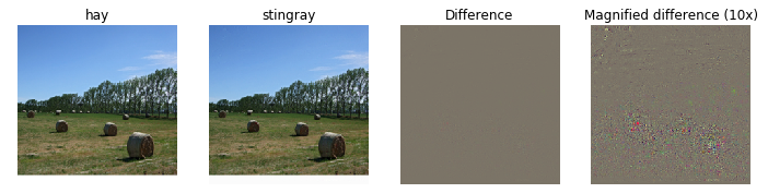
我们可以看到,欺骗图像与原始图像之间的差别非常轻微,肉眼几乎无法辨别,但是正是这种微小差异在网络进行运算之后,获得了足够使其误判的特征。
最后是类别可视化的练习,就是通过网络学习得到的特征,生成某一类别的图像。本质就是对一张随机生成的噪声图片进行梯度上升,不过和欺骗图像的区别在于这里在梯度中加入了正则项来使生成的图片更有可读性。首先是辅助函数:
def jitter(X, ox, oy):
    """
    Helper function to randomly jitter an image.

    Inputs
    - X: PyTorch Tensor of shape (N, C, H, W)
    - ox, oy: Integers giving number of pixels to jitter along W and H axes

    Returns: A new PyTorch Tensor of shape (N, C, H, W)
    """
    if ox != 0:
        left = X[:, :, :, :-ox]
        right = X[:, :, :, -ox:]
        X = torch.cat([right, left], dim=3)
    if oy != 0:
        top = X[:, :, :-oy]
        bottom = X[:, :, -oy:]
        X = torch.cat([bottom, top], dim=2)
    return X
之后就是程序本体,在欺骗图像的基础上加入了正则项:
def create_class_visualization(target_y, model, dtype, **kwargs):
    """
    Generate an image to maximize the score of target_y under a pretrained model.

    Inputs:
    - target_y: Integer in the range [0, 1000) giving the index of the class
    - model: A pretrained CNN that will be used to generate the image
    - dtype: Torch datatype to use for computations

    Keyword arguments:
    - l2_reg: Strength of L2 regularization on the image
    - learning_rate: How big of a step to take
    - num_iterations: How many iterations to use
    - blur_every: How often to blur the image as an implicit regularizer
    - max_jitter: How much to gjitter the image as an implicit regularizer
    - show_every: How often to show the intermediate result
    """
    model.type(dtype)
    l2_reg = kwargs.pop('l2_reg', 1e-3)
    learning_rate = kwargs.pop('learning_rate', 25)
    num_iterations = kwargs.pop('num_iterations', 100)
    blur_every = kwargs.pop('blur_every', 10)
    max_jitter = kwargs.pop('max_jitter', 16)
    show_every = kwargs.pop('show_every', 25)

    # Randomly initialize the image as a PyTorch Tensor, and make it requires gradient.
    img = torch.randn(1, 3, 224, 224).mul_(1.0).type(dtype).requires_grad_()

    for t in range(num_iterations):
        # Randomly jitter the image a bit; this gives slightly nicer results
        ox, oy = random.randint(0, max_jitter), random.randint(0, max_jitter)
        img.data.copy_(jitter(img.data, ox, oy))

        ########################################################################
        # TODO: Use the model to compute the gradient of the score for the     #
        # class target_y with respect to the pixels of the image, and make a   #
        # gradient step on the image using the learning rate. Don't forget the #
        # L2 regularization term!                                              #
        # Be very careful about the signs of elements in your code.            #
        ########################################################################
        score = model(img)
        loss = score[0, target_y] - l2_reg * img.norm()**2
        loss.backward()
        img.data += learning_rate * img.grad
        img.grad.zero_()
        model.zero_grad()
        ########################################################################
        #                             END OF YOUR CODE                         #
        ########################################################################

        # Undo the random jitter
        img.data.copy_(jitter(img.data, -ox, -oy))

        # As regularizer, clamp and periodically blur the image
        for c in range(3):
            lo = float(-SQUEEZENET_MEAN[c] / SQUEEZENET_STD[c])
            hi = float((1.0 - SQUEEZENET_MEAN[c]) / SQUEEZENET_STD[c])
            img.data[:, c].clamp_(min=lo, max=hi)
        if t % blur_every == 0:
            blur_image(img.data, sigma=0.5)

        # Periodically show the image
        if t == 0 or (t + 1) % show_every == 0 or t == num_iterations - 1:
            plt.imshow(deprocess(img.data.clone().cpu()))
            class_name = class_names[target_y]
            plt.title('%s\nIteration %d / %d' % (class_name, t + 1, num_iterations))
            plt.gcf().set_size_inches(4, 4)
            plt.axis('off')
            plt.show()

    return deprocess(img.data.cpu())
最后是生成图像:
dtype = torch.FloatTensor
# dtype = torch.cuda.FloatTensor # Uncomment this to use GPU
model.type(dtype)
# target_y = 76 # Tarantula
# target_y = 78 # Tick
target_y = 187 # Yorkshire Terrier
# target_y = 683 # Oboe
# target_y = 366 # Gorilla
# target_y = 604 # Hourglass
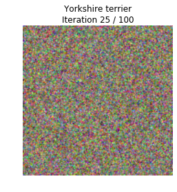
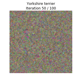
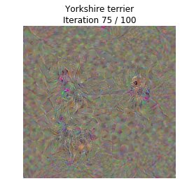
out = create_class_visualization(target_y, model, dtype)最终生成的图片如下,从最后一副图中可以看到一丢丢约克犬的影子:

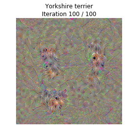
这个东西的核心用法当然不是查看网络提取的特征这么简单,它真正的意义在于:
精神污染
将上边程序中的噪声图像替换为天空图像,迭代个300代,就可以出现下面的结果:
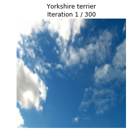

而风格迁移也是在此基础上进行改进而来的。下一篇博客将CS231n的风格迁移作业进行介绍。