译文 FaceNet: A Unified Embedding for Face Recognition and Clustering

版权声明：本文为博主原创文章，未经博主允许不得转载。 https://blog.csdn.net/chongtong/article/details/82346669

摘要

Despite significant recent advances in the field of face recognition [10, 14, 15, 17], implementing face verification and recognition efficiently at scale presents serious challenges to current approaches. In this paper we present a system, called FaceNet, that directly learns a mapping from face images to a compact Euclidean space where distances directly correspond to a measure of face similarity. Once this space has been produced, tasks such as face recognition, verification and clustering can be easily implemented using standard techniques with FaceNet embeddings as feature vectors.尽管最近在人脸识别领域取得了重大进展[10,14,15,17]，但大规模有效地实施面部验证和识别对当前方法提出了严峻挑战。 在本文中，我们提出了一个名为FaceNet的系统，它直接学习从面部图像到紧凑的欧几里德空间的映射，其中距离直接对应于面部相似性的度量。 生成此空间后，可以使用FaceNet嵌入作为特征向量的标准技术轻松实现面部识别，验证和聚类等任务。

Our method uses a deep convolutional network trained to directly optimize the embedding itself, rather than an intermediate bottleneck layer as in previous deep learning approaches. To train, we use triplets of roughly aligned matching / non-matching face patches generated using a novel online triplet mining method. The benefit of our approach is much greater representational efficiency: we achieve state-of-the-art face recognition performance using only 128-bytes per face.我们的方法使用深度卷积网络训练直接优化嵌入本身，而不是像以前的深度学习方法那样的中间瓶颈层。 为了训练，我们使用使用新颖的在线三重挖掘方法生成的大致对齐的匹配/非匹配面部补丁的三元组。 我们的方法的好处是更高的表现效率：我们使用每面只有128个字节来实现最先进的面部识别性能。

On the widely used Labeled Faces in the Wild (LFW) dataset, our system achieves a new record accuracy of 99.63%. On YouTube Faces DB it achieves 95.12%. Our system cuts the error rate in comparison to the best published result [15] by 30% on both datasets.在广泛使用的Labeled Faces in the Wild（LFW）数据集中，我们的系统实现了99.63％的新记录准确率。 在YouTube Faces DB上，它达到了95.12％。 与两个数据集中的最佳发布结果[15]相比，我们的系统将错误率降低了30％。

We also introduce the concept of harmonic embeddings, and a harmonic triplet loss, which describe different versions of face embeddings (produced by different networks) that are compatible to each other and allow for direct comparison between each other.我们还介绍了谐波嵌入和谐波三重态损耗的概念，它描述了不同版本的面嵌入（由不同网络产生），它们彼此兼容并允许彼此之间的直接比较。

1. 介绍

In this paper we present a unified system for face verification (is this the same person), recognition (who is this person) and clustering (find common people among these faces). Our method is based on learning a Euclidean embedding per image using a deep convolutional network. The network is trained such that the squared L2 distances in the embedding space directly correspond to face similarity: faces of the same person have small distances and faces of distinct people have large distances.在本文中，我们提出了一个统一的面部验证系统（在这里是指同一个人），识别（谁是这个人）和聚类（在这些面孔中找到相同的人）。 我们的方法基于使用深度卷积网络学习每个图像的欧几里德嵌入。 训练网络使得嵌入空间中的平方L2距离直接对应于面部相似性：同一人的面部具有小距离并且不同人的面部具有大距离。

Once this embedding has been produced, then the aforementioned tasks become straight-forward: face verification simply involves thresholding the distance between the two embeddings; recognition becomes a k-NN classification problem; and clustering can be achieved using off-theshelf techniques such as k-means or agglomerative clustering.一旦产生了这种嵌入，则上述任务变得直截了当：面部验证仅涉及对两个嵌入之间的距离进行阈值处理; 识别任务成为k-NN分类问题; 并且可以使用诸如k均值或凝聚聚类之类的现有技术来实现聚类。

Previous face recognition approaches based on deep networks use a classification layer [15, 17] trained over a set of known face identities and then take an intermediate bottle-neck layer as a epresentation used to generalize recognition beyond the set of identities used in training. The downsides of this approach are its indirectness and its inefficiency: one has to hope that the bottleneck representation generalizes well to new faces; and by using a bottleneck layer the representation size per face is usually very large (1000s of dimensions). Some recent work [15] has reduced this dimensionality using PCA, but this is a linear transformation that can be easily learnt in one layer of the network.先前基于深度网络的面部识别方法使用在一组已知面部身份上训练的分类层[15,17]，然后采用中间瓶颈层作为表示，用于概括超出训练中使用的身份集合的识别。 这种方法的缺点是它的间接性和效率低下：人们不得不希望瓶颈表现能够很好地概括为新面孔; 通过使用瓶颈层，每个面的表示大小通常非常大（1000维）。 最近的一些工作[15]使用PCA降低了这种维度，但这是一种线性转换，可以在网络的一个层中轻松学习。

In contrast to these approaches, FaceNet directly trains its output to be a compact 128-D embedding using a tripletbased loss function based on LMNN [19]. Our triplets consist of two matching face thumbnails and a non-matching face thumbnail and the loss aims to separate the positive pair from the negative by a distance margin. The thumbnails are tight crops of the face area, no 2D or 3D alignment, other than scale and translation is performed.与这些方法相比，FaceNet直接将其输出训练为使用基于LMNN的使用三重损耗函数的紧凑128-D嵌入[19]。 我们的三元组由两个匹配的面部缩略图和一个不匹配的面部缩略图组成，并且损失的目标是将正对与负对分开一个距离边距。 缩略图是面部区域的紧密裁剪，除了缩放和平移之外，没有2D或3D对齐。

Choosing which triplets to use turns out to be very important for achieving good performance and, inspired by curriculum learning [1], we present a novel online negative exemplar mining strategy which ensures consistently increasing difficulty of triplets as the network trains. To improve clustering accuracy, we also explore hard-positive mining techniques which encourage spherical clusters for the embeddings of a single person.选择使用哪些三元组对于实现良好的表现非常重要，并且受Curriculum learning的启发[1]，我们提出了一种新颖的在线负面样本挖掘策略，确保在网络训练时不断增加三元组的难度。 为了提高聚类精度，我们还探索了硬阳性挖掘技术，该技术鼓励球形聚类用于嵌入单个人。

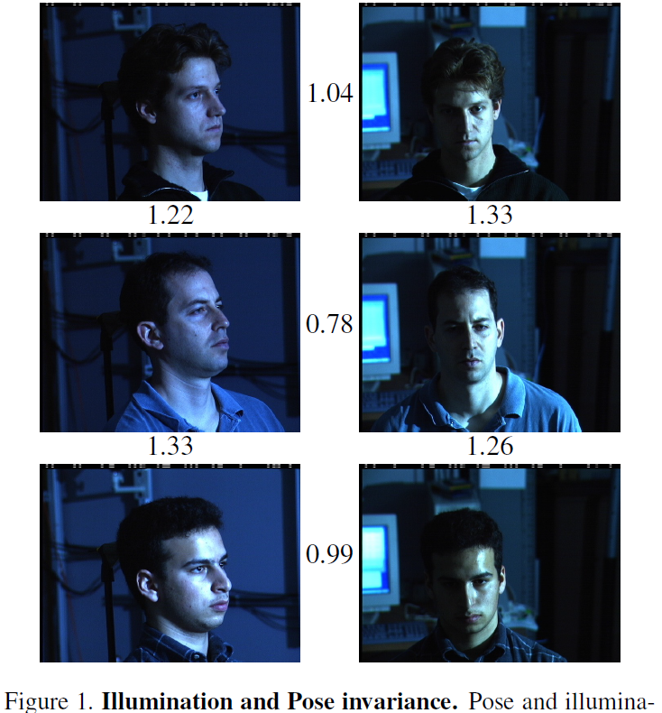
Figure 1. Illumination and Pose invariance. Pose and illumination have been a long standing problem in face recognition. This figure shows the output distances of FaceNet between pairs of faces of the same and a different person in different pose and illumination combinations. A distance of 0:0 means the faces are identical, 4:0 corresponds to the opposite spectrum, two different identities. You can see that a threshold of 1.1 would classify every pair correctly.图1.照明和姿势不变性。 姿势和照明是人脸识别中长期存在的问题。 该图显示了FaceNet在不同姿势和照明组合中相同和不同人的面对之间的输出距离。 距离0.0表示面相同，4.0对应相反的光谱，两个不同的身份。 您可以看到1.1的阈值会正确地对每一对进行分类。

As an illustration of the incredible variability that our method can handle see Figure 1. Shown are image pairs from PIE [13] that previously were considered to be very difficult for face verification systems.作为我们的方法可以处理的令人难以置信的可变性的说明，请参见图1.显示来自PIE [13]的图像对，之前被认为对于面部验证系统来说非常困难。

An overview of the rest of the paper is as follows: in section 2 we review the literature in this area; section 3.1 defines the triplet loss and section 3.2 describes our novel triplet selection and training procedure; in section 3.3 we describe the model architecture used. Finally in section 4 and 5 we present some quantitative results of our embeddings and also qualitatively explore some clustering results.本文其余部分的概述如下：在第2节中，我们回顾了该领域的文献; 第3.1节定义了三重态损失，第3.2节描述了我们新颖的三重态选择和训练程序; 在3.3节中，我们描述了使用的模型架构。 最后在第4节和第5节中，我们提供了嵌入的一些定量结果，并定性地探索了一些聚类结果。

2. 相关工作

Similarly to other recent works which employ deep networks [15, 17], our approach is a purely data driven method which learns its representation directly from the pixels of the face. Rather than using engineered features, we use a large dataset of labelled faces to attain the appropriate invariances to pose, illumination, and other variational conditions.与其他最近使用深度网络的作品[15,17]类似，我们的方法是一种纯粹的数据驱动方法，它直接从面部像素中学习它的表示。 我们使用标记过人脸的大型数据集来获得姿势，光照和其他变化条件的适当不变性，而不是使用工程特征。

In this paper we explore two different deep network architectures that have been recently used to great success in the computer vision community. Both are deep convolutional networks [8, 11]. The first architecture is based on the Zeiler&Fergus [22] model which consists of multiple interleaved layers of convolutions, non-linear activations, local response normalizations, and max pooling layers. We additionally add several 11d convolution layers inspired by the work of [9]. The second rchitecture is based on the Inception model of Szegedy et al. which was recently used as the winning approach for ImageNet 2014 [16]. These networks use mixed layers that run several different convolutional and pooling layers in parallel and concatenate their responses. We have found that these models can reduce the number of parameters by up to 20 times and have the potential to reduce the number of FLOPS required for comparable performance.在本文中，我们探讨了最近在计算机视觉社区中取得巨大成功的两种不同的深度网络架构。 两者都是深度卷积网络[8,11]。 第一种架构基于Zeiler＆Fergus [22]模型，该模型由多个交错的卷积层，非线性激活，局部响应归一化和最大池化层组成。 我们还增加了几个1*1*d卷积层，灵感来自[9]的工作。 第二种结构基于Szegedy等人的Inception模型。 最近被用作ImageNet 2014的获胜方法[16]。 这些网络使用混合层，并行运行几个不同的卷积和池化层并连接它们的响应。 我们发现这些模型可以将参数数量减少多达20倍，并且有可能减少可比性能所需的FLOPS数量。

There is a vast corpus of face verification and recognition works. Reviewing it is out of the scope of this paper so we will only briefly discuss the most relevant recent work.目前有大量的面部验证和识别工作。 审查它超出了本文的范围，因此我们将仅简要讨论最相关的最新工作。

The works of [15, 17, 23] all employ a complex system of multiple stages, that combines the output of a deep convolutional network with PCA for dimensionality reduction and an SVM for classification.论文[15,17,23]都使用了一个复杂的多级系统，它将深度卷积网络的输出与PCA相结合，以降低维数，并将SVM用于分类。

Zhenyao et al. [23] employ a deep network to “warp” faces into a canonical frontal view and then learn CNN that classifies each face as belonging to a known identity. For face verification, PCA on the network output in conjunction with an ensemble of SVMs is used.Zhenyao等 [23]采用深度网络将面部“扭曲”成规范的正面视图，然后学习CNN，将每个面部分类为属于已知身份。 对于面部验证，使用网络输出上的PCA和一组SVM。

Taigman et al. [17] propose a multi-stage approach that aligns faces to a general 3D shape model. A multi-class network is trained to perform the face recognition task on over four thousand identities. The authors also experimented with a so called Siamese network where they directly optimize the L1-distance between two face features. Their best performance on LFW (97:35%) stems from an ensemble of three networks using different alignments and color channels. The predicted distances (non-linear SVM predictions based on the 2 kernel) of those networks are combined using a non-linear SVM.Taigman等 [17]提出了一种多阶段方法，将面部与一般的三维形状模型对齐。 训练多级网络以执行超过四千个特征的面部识别任务。 作者还试验了一个所谓的连体网络，他们直接优化了两个面部特征之间的L1距离。 他们在LFW上的最佳表现（97.35％）源于使用不同比对和颜色通道的三个网络的集合。 使用非线性SVM组合这些网络的预测距离（基于α2内核的非线性SVM预测）。

Sun et al. [14, 15] propose a compact and therefore relatively cheap to compute network. They use an ensemble of 25 of these network, each operating on a different face patch. For their final performance on LFW (99:47% [15]) the authors combine 50 responses (regular and flipped). Both PCA and a Joint Bayesian model [2] that effectively correspond to a linear transform in the embedding space are employed. Their method does not require explicit 2D/3D alignment. The networks are trained by using a combination of classification and verification loss. The verification loss is similar to the triplet loss we employ [12, 19], in that it minimizes the L2-distance between faces of the same identity and enforces a margin between the distance of faces of different identities. The main difference is that only pairs of images are compared, whereas the triplet loss encourages a relative distance constraint.孙等 [14,15]提出了一种紧凑且因此相对便宜的计算网络。 他们使用25个这样的网络集合，每个网络在不同的面部补丁上运行。 对于他们在LFW上的最终表现（99：47％[15]），作者结合了50个回答（常规和翻转）。 PCA和联合贝叶斯模型[2]都有效地对应于嵌入空间中的线性变换。 他们的方法不需要明确的2D / 3D对齐。 通过使用分类和验证丢失的组合损失函数来训练网络。 验证损失函数类似于我们采用的三元组损失[12,19]，因为它最小化了相同身份的面部之间的L2距离，并在不同身份的面部距离之间实施了边界。 主要区别在于仅比较成对图像，而三元组损失促使相对距离约束。

A similar loss to the one used here was explored in Wang et al. [18] for ranking images by semantic and visual similarity.Wang等人研究了与此处使用的类似的损失。 [18]用于通过语义和视觉相似性对图像进行排序。

3. 方法

FaceNet uses a deep convolutional network. We discuss two different core architectures: The Zeiler&Fergus [22] style networks and the recent Inception [16] type networks. The details of these networks are described in section 3.3.FaceNet使用深度卷积网络。 我们讨论了两种不同的核心架构：Zeiler＆Fergus [22]式网络和最近的Inception [16]型网络。 这些网络的细节在3.3节中描述。

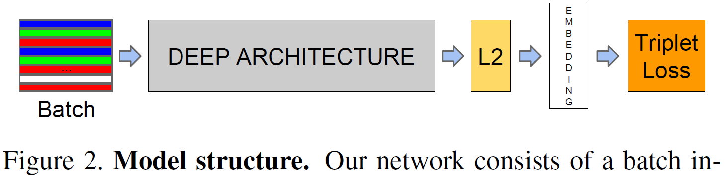
Figure 2. Model structure. Our network consists of a batch input layer and a deep CNN followed by L2 normalization, which results in the face embedding. This is followed by the triplet loss during training.图2.模型结构。 我们的网络由批量输入层和深度CNN组成，然后进行L2归一化，从而实现面嵌入。 接下来是训练期间的三元组损失。

Given the model details, and treating it as a black box (see Figure 2), the most important part of our approach lies in the end-to-end learning of the whole system. To this end we employ the triplet loss that directly reflects what we want to achieve in face verification, recognition and clustering. Namely, we strive for an embedding f(x), from an image x into a feature space Rd, such that the squared distance between all faces, independent of imaging conditions, of the same identity is small, whereas the squared distance between a pair of face images from different identities is large.将模型细节视为黑盒子（见图2），我们方法中最重要的部分在于整个系统的端到端学习。 为此，我们采用三元组损失，直接反映了我们想要在面部验证，识别和聚类中实现的目标。 即，我们努力嵌入f（x），从图像x到特征空间Rd，使得相同身份的所有面之间的平方距离（与成像条件无关）很小，而一对之间的平方距离很小。 来自不同身份的面部图像很大。

Although we did not directly compare to other losses, e.g. the one using pairs of positives and negatives, as used in [14] Eq. (2), we believe that the triplet loss is more suitable for face verification. The motivation is that the loss from [14] encourages all faces of one identity to be projected onto a single point in the embedding space. The triplet loss, however, tries to enforce a margin between each pair of faces from one person to all other faces. This allows the faces for one identity to live on a manifold, while still enforcing the distance and thus discriminability to other identities.虽然我们没有直接与其他损失进行比较，例如 使用[14] Eq中使用的正和负对的那个。 （2），我们认为三联体损失更适合面部识别。 动机是[14]的损失鼓励将一个身份的所有面部投射到嵌入空间中的单个点上。 然而，三重态损失试图在从一个人到所有其他面部的每对面部之间强制执行边缘。 这允许一个身份的面部应用在个人的多样上，同时仍然强制距离并因此可以与其他身份相区别。

The following section describes this triplet loss and how it can be learned efficiently at scale.以下部分描述了这种三元组损失以及如何有效地大规模学习它。

3.1. 三元组损失

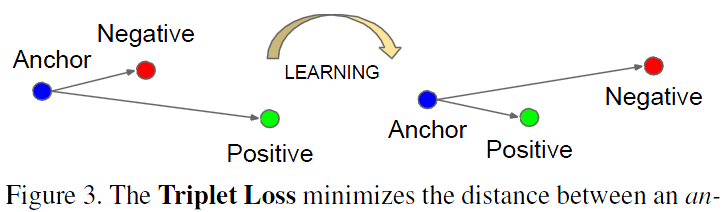
Figure 3. The Triplet Loss minimizes the distance between an anchor and a positive, both of which have the same identity, and maximizes the distance between the anchor and a negative of a different identity.图3.三联体损失最小化锚和阳性之间的距离，两者具有相同的身份，并最大化锚和不同身份的阴性之间的距离。

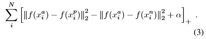
The embedding is represented by f(x) 2 Rd. It embeds an image x into a d-dimensional Euclidean space. Additionally, we constrain this embedding to live on the d-dimensional hypersphere, i.e. kf(x)k2 = 1. This loss is motivated in [19] in the context of nearest-neighbor classification. Here we want to ensure that an image xai (anchor) of a specific person is closer to all other images xpi (positive) of the same person than it is to any image xni (negative) of any other person. This is visualized in Figure 3.嵌入由f（x）2 Rd表示。 它将图像x嵌入到d维欧几里德空间中。 另外，我们将这种嵌入限制在d维超球面上，即kf（x）k2 = 1.这种损失在[19]中在最近邻分类的背景下被激发。 在这里，我们希望确保特定人的图像xai（锚）更接近同一个人的所有其他图像xpi（正面），而不是任何其他人的任何图像xni（负面）。 见图3中的图示。因此

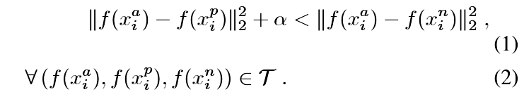
where a is a margin that is enforced between positive and negative pairs. T is the set of all possible triplets in the training set and has cardinality N.在公式里a是正负对之间区分界限的阈值。 T是训练集中所有可能的三元组的集合，并具有基数N.损失函数定义为

Generating all possible triplets would result in many triplets that are easily satisfied (i.e. fulfill the constraint in Eq. (1)). These triplets would not contribute to the training and result in slower convergence, as they would still be passed through the network. It is crucial to select hard triplets, that are active and can therefore contribute to improving the model. The following section talks about the different approaches we use for the triplet selection.生成所有可能的三元组将导致许多容易满足的三元组（即满足方程（1）中的约束）。 这些三元组不会对训练有所贡献，导致收敛速度变慢，因为它们仍会通过网络传递。 选择活跃的硬三元组至关重要，因此可以有助于改进模型。 下一节讨论了我们用于三元组选择的不同方法。

3.2. 三元组的选择

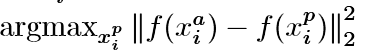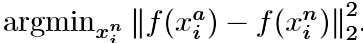In order to ensure fast convergence it is crucial to select triplets that violate the triplet constraint in Eq. (1). This means that, given xai, we want to select an xpi (hard positive) such that fff and similarly xni(hard negative) such that ddd。为了确保快速收敛，选择违反方程式（1）中的三元组约束的三元组是至关重要的。 这意味着，对于给定的xai，我们需要选择一个xpi（硬正）和xni（硬阴性），使得和接近。

It is infeasible to compute the argmin and argmax across the whole training set. Additionally, it might lead to poor training, as mislabelled and poorly imaged faces would dominate the hard positives and negatives. There are two obvious choices that avoid this issue:在整个训练集中计算argmin和argmax是不可行的。 此外，它可能导致训练不佳，因为错误标记和不良成像的面孔将主导硬性积极和消极。 有两个明显的选择可以避免这个问题：
- Generate triplets offline every n steps, using the most recent network checkpoint and computing the argmin and argmax on a subset of the data.使用最新的网络检查点并在数据的子集上计算argmin和argmax，每n个步骤生成三元组。
- Generate triplets online. This can be done by selecting the hard positive/negative exemplars from within a mini-batch.在线生成三元组。 这可以通过从小批量中选择硬正/负样本来完成。

Here, we focus on the online generation and use large mini-batches in the order of a few thousand exemplars and only compute the argmin and argmax within a mini-batch.在这里，我们专注于在线生成并使用大约几千个样本的大型小批量，并且仅在小批量中计算argmin和argmax。

To have a meaningful representation of the anchorpositive distances, it needs to be ensured that a minimal number of exemplars of any one identity is present in each mini-batch. In our experiments we sample the training data such that around 40 faces are selected per identity per minibatch. Additionally, randomly sampled negative faces are added to each mini-batch.为了有效地表示锚定距离，需要确保每个小批量中存在任何一个身份的最小数量的样本。 在我们的实验中，我们对训练数据进行采样，使得每个小批量每个身份选择约40个面部。 另外，随机抽样的负面被添加到每个小批量。

Instead of picking the hardest positive, we use all anchorpositive pairs in a mini-batch while still selecting the hard negatives. We don’t have a side-by-side comparison of hard anchor-positive pairs versus all anchor-positive pairs within a mini-batch, but we found in practice that the all anchorpositive method was more stable and converged slightly faster at the beginning of training.我们不是挑选最差的正样本，而是在小批量中使用所有正样本锚定对，同时仍然选择硬阴性。 我们没有对一个小批次中的硬锚阳性对与所有锚 - 阳对进行并排比较，但我们在实践中发现所有锚定阳性方法在开始时更稳定并且收敛得稍快一些 训练。

We also explored the offline generation of triplets in conjunction with the online generation and it may allow the use of smaller batch sizes, but the experiments were inconclusive.我们还与在线生成一起探索了三联体的离线生成，并且可能允许使用更小的批量，但实验尚无定论。

Selecting the hardest negatives can in practice lead to bad local minima early on in training, specifically it can result in a collapsed model (i.e. f(x) = 0). In order to mitigate this, it helps to select xni such that选择最难的负样本实际上可能在训练早期导致不良的局部最小值，特别是它可能导致模型崩溃（如f（x）= 0）。 为了减轻这种影响，用如下条件选择xni会有所帮助

We call these negative exemplars semi-hard, as they are further away from the anchor than the positive exemplar, but still hard because the squared distance is close to the anchorpositive distance. Those negatives lie inside the margin .我们将这些负面样本称为半硬，因为它们远离锚点而不是正样本，但仍然很难，因为平方距离接近锚定距离。 这些负面影响在阈值范围内。

As mentioned before, correct triplet selection is crucial for fast convergence. On the one hand we would like to use small mini-batches as these tend to improve convergence during Stochastic Gradient Descent (SGD) [20]. On the other hand, implementation details make batches of tens to hundreds of exemplars more efficient. The main constraint with regards to the batch size, however, is the way we select hard relevant triplets from within the mini-batches. In most experiments we use a batch size of around 1,800 exemplars.如前所述，正确的三元组选择对于快速收敛至关重要。 一方面，我们希望使用小型小批量，因为这些趋向于在随机梯度下降（SGD）期间改善收敛[20]。 另一方面，实施细节使得数十到数百个样本的批次更有效。 然而，关于批量大小的主要限制是我们从小批量中选择硬相关三元组的方式。 在大多数实验中，我们使用的批量大小约为1,800个样本。

3.3. 深度卷积网络

In all our experiments we train the CNN using Stochastic Gradient Descent (SGD) with standard backprop [8, 11] and AdaGrad [5]. In most experiments we start with a learning rate of 0:05 which we lower to finalize the model. The models are initialized from random, similar to [16], and trained on a CPU cluster for 1,000 to 2,000 hours. The decrease in the loss (and increase in accuracy) slows down drastically after 500h of training, but additional training can still significantly improve performance. The margin a is set to 0:2.在我们的所有实验中，我们使用随机梯度下降（SGD）的标准反向传播[8,11]和AdaGrad [5]训练CNN。 在大多数实验中，我们从学习率0.05开始，我们降低以完成模型。 模型从随机初始化，类似于[16]，并在CPU集群上训练1,000到2,000小时。 在训练500小时后，损失的减少（以及准确度的增加）急剧减慢，但额外的训练仍然可以显着提高性能。 边距a设置为0.2。

We used two types of architectures and explore their trade-offs in more detail in the experimental section. Their practical differences lie in the difference of parameters and FLOPS. The best model may be different depending on the application. E.g. a model running in a datacenter can have many parameters and require a large number of FLOPS, whereas a model running on a mobile phone needs to have few parameters, so that it can fit into memory. All our models use rectified linear units as the non-linear activation function.我们使用了两种类型的体系结构，并在实验部分中更详细地探讨了它们的权衡。 它们的实际差异在于参数和FLOPS的差异。 根据应用，最佳型号可能会有所不同。 例如。 在数据中心中运行的模型可以具有许多参数并且需要大量FLOPS，而在移动电话上运行的模型需要具有很少的参数，以便它可以适合存储器。 我们所有的模型都使用整流线性单元（RELU）作为非线性激活函数。

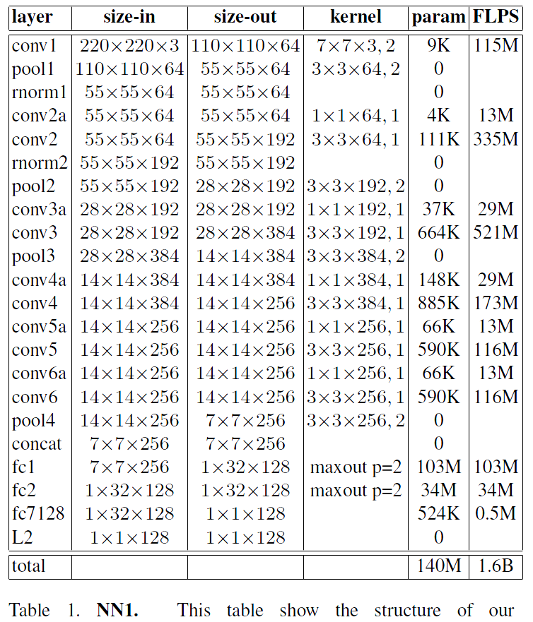
Table 1. NN1. This table show the structure of our Zeiler&Fergus [22] based model with 1*1 convolutions inspired by [9]. The input and output sizes are described in rows*cols*#filters. The kernel is specified as rows*cols; stride and the maxout [6] pooling size as p = 2.表1. NN1。 该表显示了我们的Zeiler＆Fergus [22]模型的结构，其灵感来自于[9]的1*1卷积。 输入和输出大小描述为 rows*cols*#filters。 内核被指定为rows*cols; 步幅和maxout [6]的池化大小为p = 2。

The first category, shown in Table 1, adds 11d convolutional layers, as suggested in [9], between the standard convolutional layers of the Zeiler&Fergus [22] architecture and results in a model 22 layers deep. It has a total of 140 million parameters and requires around 1.6 billion FLOPS per image.第一类结构，如表1所示，如[9]中建议，在Zeiler＆Fergus [22]架构的标准卷积层之间增加1*1*d卷积层，得到22层深的模型。 它总共有1.4亿个参数，每个图像需要大约16亿FLOPS。

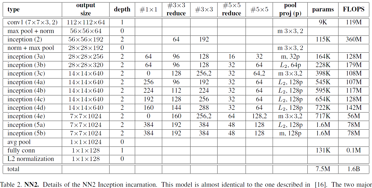
Table 2. NN2. Details of the NN2 Inception incarnation. This model is almost identical to the one described in [16]. The two major differences are the use of L2 pooling instead of max pooling (m), here specified. I.e. instead of taking the spatial max the L2 norm is computed. The pooling is always 33 (aside from the final average pooling) and in parallel to the convolutional modules inside each Inception module. If there is a dimensionality reduction after the pooling it is denoted with p. 11, 33, and 55 pooling are then concatenated to get the final output.表2.NN2。 NN2 Inception 实现的详细信息。 该模型几乎与[16]中描述的模型相同。 两个主要区别是使用L2池化而不是最大池化（m），这里指定。即不是取空间最大值，而是计算L2范数。 池化窗总是3*3（除了最终的平均池化），并且与每个Inception模块内的卷积模块并行。 如果在池化后存在降维，则用p表示。 然后连接1*1,3*3和5*5池化会汇集以获得最终输出。

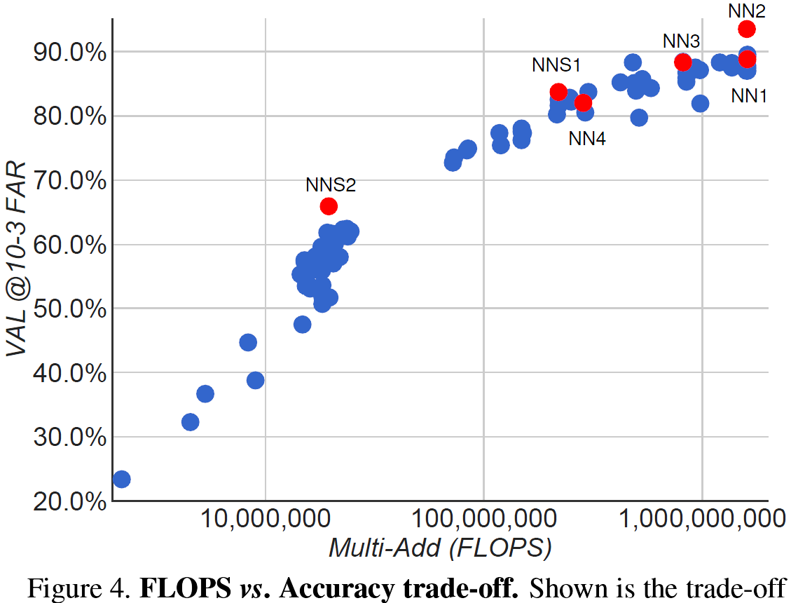
Figure 4. FLOPS vs. Accuracy trade-off. Shown is the trade-off between FLOPS and accuracy for a wide range of different model sizes and architectures. Highlighted are the four models that we focus on in our experiments.图4. FLOPS与准确性的权衡。 所示为FLOPS与各种不同型号和架构的精度之间的权衡。 重点介绍了我们在实验中关注的四种模型。

The second category we use is based on GoogLeNet style Inception models [16]. These models have 20* fewer parameters (around 6.6M-7.5M) and up to 5fewer FLOPS (between 500M-1.6B). Some of these models are dramatically reduced in size (both depth and number of filters), so that they can be run on a mobile phone. One, NNS1, has 26M parameters and only requires 220M FLOPS per image. The other, NNS2, has 4.3M parameters and 20M FLOPS. Table 2 describes NN2 our largest network in detail. NN3 is identical in architecture but has a reduced input size of 160x160. NN4 has an input size of only 96x96, thereby drastically reducing the CPU requirements (285M FLOPS vs 1.6B for NN2). In addition to the reduced input size it does not use 5x5 convolutions in the higher layers as the receptive field is already too small by then. Generally we found that the 5x5 convolutions can be removed throughout with only a minor drop in accuracy. Figure 4 compares all our models.我们使用的第二类是基于GoogLeNet风格的Inception模型组[16]。 部分模型使参数减少20倍（约6.6M-7.5M），FLOPS减少5倍（500M-1.6B之间）。 其中一些型号的尺寸（深度和滤波器数量）都大幅减少，因此可以在手机上运行。 一，NNS1，具有26M参数，每个图像仅需要220M FLOPS。 另一个是NNS2，有4.3M参数和20M FLOPS。 表2详细描述了我们最大的网络NN2。 NN3在架构上是相同的，但输入尺寸减小了160x160。 NN4的输入大小仅为96x96，从而大幅降低了CPU要求（NN2为285M FLOPS对1.6B）。 除了减小的输入尺寸之外，它在较高层中不使用5x5卷积，因为此时感受野已经太小。 一般来说，我们发现5x5卷积可以在整个过程中被移除，只有很小的精度下降。 图4比较了我们所有的模型。

4. 数据集和评估

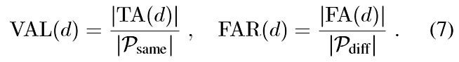
We evaluate our method on four datasets and with the exception of Labelled Faces in the Wild and YouTube Faces we evaluate our method on the face verification task. I.e. given a pair of two face images a squared L2 distance threshold D(xi; xj) is used to determine the classification of same and different. All faces pairs (i; j) of the same identity are denoted with Psame, whereas all pairs of different identities are denoted with Pdiff.我们在四个数据集上评估我们的方法，除了Wild和YouTube Faces中的Labeled Faces，我们在面部验证任务上评估我们的方法。即 给定一对两个面部图像，使用平方L2距离阈值D（xi; xj）来确定相同和不同的分类。 具有相同身份的所有面部对（i; j）用Psame表示，而所有不同身份对用Pdiff表示。我们定义TA和FA为：

The validation rate VAL(d) and the false accept rate FAR(d) for a given face distance d are then defined as然后将在给定面部距离d下的验证率VAL（d）和错误接受率FAR（d）定义为

4.1. 保持测试集

We keep a hold out set of around one million images, that has the same distribution as our training set, but disjoint identities. For evaluation we split it into five disjoint sets of 200k images each. The FAR and VAL rate are then computed on 100k*100k image pairs. Standard error is reported across the five splits.我们保留了大约一百万张图像，与我们的训练集具有相同的分布，但不相同的身份。 为了评估，我们将它分成五个不相交的数据集，每组200k图像。 然后在100k*100k的图像对上计算FAR和VAL率。 在五个数据集的结果中报告标准错误。

4.2. 个人照片

This is a test set with similar distribution to our training set, but has been manually verified to have very clean labels. It consists of three personal photo collections with a total of around 12k images. We compute the FAR and VAL rate across all 12k squared pairs of images.这是一个与我们的训练集具有类似分布的测试集，但已经过手动验证，具有非常干净的标签。 它由三个个人照片集合组成，总共大约12k图像。 我们计算所有12k平方对图像的FAR和VAL率。

4.3. 学术数据集

Labeled Faces in the Wild (LFW) is the de-facto academic test set for face verification [7]. We follow the standard protocol for unrestricted, labeled outside data and report the mean classification accuracy as well as the standard error of the mean.野外标记面（LFW）是面部验证的事实上的学术测试集[7]。 我们遵循标准协议，对无限制，标记的外部数据进行报告，并报告平均分类准确度以及均值的标准误差。

Youtube Faces DB [21] is a new dataset that has gained popularity in the face recognition community [17, 15]. The setup is similar to LFW, but instead of verifying pairs of images, pairs of videos are used.Youtube Faces DB [21]是一个新的数据集，在人脸识别领域得到了普及[17,15]。 该设置类似于LFW，但不使用验证图像对，而是使用视频对。

5. 实验

If not mentioned otherwise we use between 100M-200M training face thumbnails consisting of about 8M different identities. A face detector is run on each image and a tight bounding box around each face is generated. These face thumbnails are resized to the input size of the respective network. Input sizes range from 96x96 pixels to 224x224 pixels in our experiments.如果没有提到，否则我们使用100M-200M训练面部缩略图，其中包含大约8M个不同的身份。 在每个图像上运行面部检测器，并且生成围绕每个面的紧密边界框。 这些面部缩略图的大小调整为相应网络的输入大小。 在我们的实验中，输入尺寸范围从96x96像素到224x224像素。

5.1. 计算准确性权衡

Before diving into the details of more specific experiments we will discuss the trade-off of accuracy versus number of FLOPS that a particular model requires. Figure 4 shows the FLOPS on the x-axis and the accuracy at 0.001 false accept rate (FAR) on our user labelled test-data set from section 4.2. It is interesting to see the strong correlation between the computation a model requires and the accuracy it achieves. The figure highlights the five models (NN1, NN2, NN3, NNS1, NNS2) that we discuss in more detail in our experiments.在深入了解更具体的实验细节之前，我们将讨论精确度与特定模型所需的FLOPS数量之间的权衡。 图4显示了x轴上的FLOPS以及4.2节中用户标记的测试数据集的0.001错误接受率（FAR）的准确度。 有趣的是，模型所需的计算与其实现的精度之间存在很强的相关性。 该图突出显示了我们在实验中更详细讨论的五个模型（NN1，NN2，NN3，NNS1，NNS2）。

We also looked into the accuracy trade-off with regards to the number of model parameters. However, the picture is not as clear in that case. For example, the Inception based model NN2 achieves a comparable performance to NN1, but only has a 20th of the parameters. The number of FLOPS is comparable, though. Obviously at some point the performance is expected to decrease, if the number of parameters is reduced further. Other model architectures may allow further reductions without loss of accuracy, just like Inception [16] did in this case.我们还研究了关于模型参数数量的准确性权衡。 但是，在这种情况下，情况并不那么清楚。 例如，基于Inception的模型NN2实现了与NN1相当的性能，但只有20个参数。 但是，FLOPS的数量是可比的。 显然，如果参数的数量进一步减少，预计性能会下降。 其他模型架构可以允许进一步减少而不会损失准确性，就像Inception [16]在这种情况下所做的那样。

5.2. CNN模型的效果

We now discuss the performance of our four selected models in more detail. On the one hand we have our traditional Zeiler&Fergus based architecture with 11 convolutions [22, 9] (see Table 1). On the other hand we have Inception [16] based models that dramatically reduce the model size. Overall, in the final performance the top models of both architectures perform comparably. However, some of our Inception based models, such as NN3, still achieve good performance while significantly reducing both the FLOPS and the model size.我们现在更详细地讨论我们四个选定模型的性能。 一方面，我们采用传统的基于Zeiler和Fergus的架构，具有1*1卷积[22,9]（见表1）。 另一方面，我们有基于Inception [16]的模型，可以大大减少模型的大小。 总的来说，在最终的表现中，两种架构的顶级模型表现相当。 但是，我们的一些基于Inception的模型（如NN3）仍然可以实现良好的性能，同时显着降低FLOPS和模型大小。

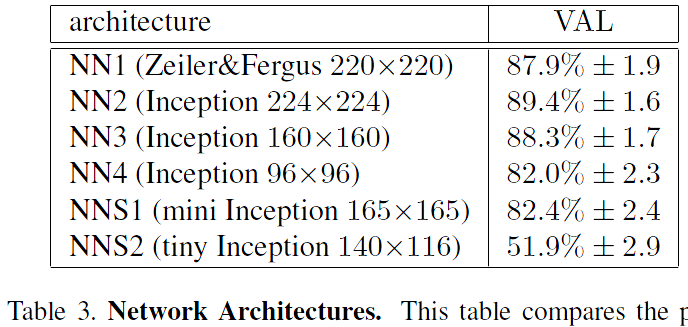
Table 3. Network Architectures. This table compares the performance of our model architectures on the hold out test set (see section 4.1). Reported is the mean validation rate VAL at 10E-3 false accept rate. Also shown is the standard error of the mean across the five test splits.表3.网络体系结构。 该表比较了我们的模型架构在保持测试集上的性能（参见第4.1节）。 报告的是10E-3错误接受率下的平均验证率VAL。 还显示了五个测试分裂中的平均值的标准误差。

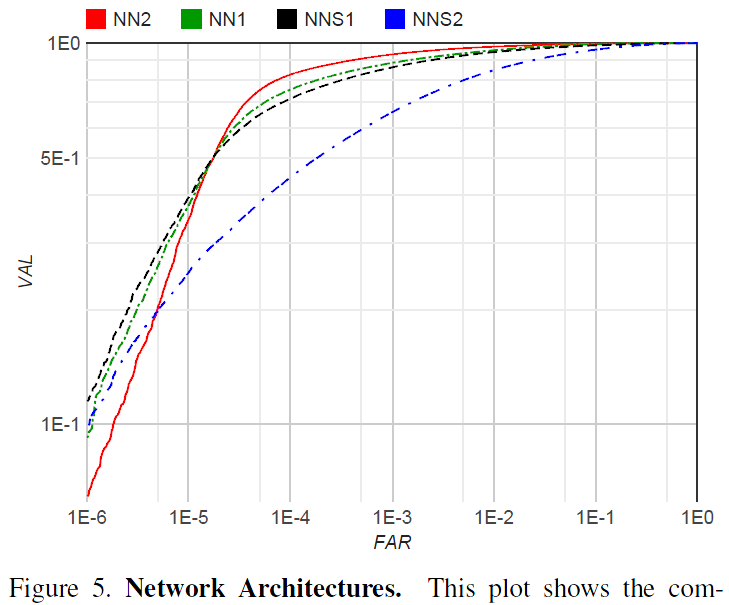
Figure 5. Network Architectures. This plot shows the complete ROC for the four different models on our personal photos test set from section 4.2. The sharp drop at 10E-4 FAR can be explained by noise in the groundtruth labels. The models in order of performance are: NN2: 224224 input Inception based model; NN1: Zeiler&Fergus based network with 11 convolutions; NNS1: small Inception style model with only 220M FLOPS; NNS2: tiny Inception model with only 20M FLOPS.图5.网络架构 该图显示了4.2节中我们个人照片测试集中四种不同模型的完整ROC。 10E-4 FAR的急剧下降可以通过groundtruth标签中的噪声来解释。 性能顺序为：NN2：224*224输入基于初始的模型; NN1：基于Zeiler＆Fergus的网络，1*1卷积; NNS1：小型Inception风格型号，仅有220M FLOPS; NNS2：微小的Inception模型，只有20M FLOPS。

The detailed evaluation on our personal photos test set is shown in Figure 5. While the largest model achieves a dramatic improvement in accuracy compared to the tiny NNS2, the latter can be run 30ms / image on a mobile phone and is still accurate enough to be used in face clustering. The sharp drop in the ROC for FAR < 10e-4 indicates noisy labels in the test data groundtruth. At extremely low false accept rates a single mislabeled image can have a significant impact on the curve.我们的个人照片测试装置的详细评估如图5所示。虽然最小的型号与小型NNS2相比可以显着提高精度，后者可以在手机上运行30ms /图像，并且仍然足够准确 用于面部聚类。 FAR \<10e-4的ROC急剧下降表明测试数据中的标签噪声很大。 在极低的错误接受率下，单个错误标记的图像会对曲线产生显着影响。

5.3. 对图片质量的敏感度

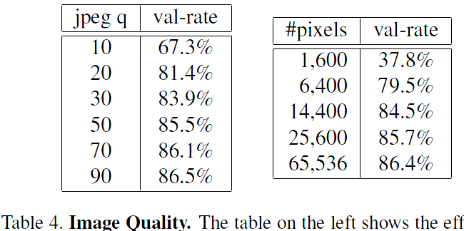
Table 4. Image Quality. The table on the left shows the effect on the validation rate at 10E-3 precision with varying JPEG quality. The one on the right shows how the image size in pixels effects the validation rate at 10E-3 precision. This experiment was done with NN1 on the first split of our test hold-out dataset.表4.图像质量。 左侧的表格显示了不同JPEG质量对10E-3精度的验证率的影响。 右边的那个显示图像大小（以像素为单位）如何影响10E-3精度的验证率。 在我们的测试保持数据集的第一次拆分中，使用NN1完成了该实验。

Table 4 shows the robustness of our model across a wide range of image sizes. The network is surprisingly robust with respect to JPEG compression and performs very well down to a JPEG quality of 20. The performance drop is very small for face thumbnails down to a size of 120x120 pixels and even at 80x80 pixels it shows acceptable performance. This is notable, because the network was trained on 220x220 input images. Training with lower resolution faces could improve this range further.表4显示了我们的模型在各种图像尺寸上的稳健性。 该网络在JPEG压缩方面非常强大，并且在JPEG质量为20时表现非常好。对于尺寸为120x120像素的面部缩略图，性能下降非常小，即使在80x80像素下也表现出可接受的性能。 这是值得注意的，因为网络是在220x220输入图像上训练的。 低分辨率面部训练可以进一步改善这个范围。

5.4. 嵌入维度

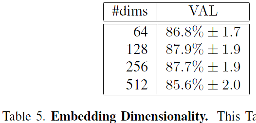
Table 5. Embedding Dimensionality. This Table compares the effect of the embedding dimensionality of our model NN1 on our hold-out set from section 4.1. In addition to the VAL at 10E-3 we also show the standard error of the mean computed across five splits.表5.嵌入维度。 该表比较了我们的模型NN1的嵌入维数对4.1节中的保持集的影响。 除了在10E-3处的VAL之外，我们还显示了在五个子数据集中计算的平均值的标准误差。

We explored various embedding dimensionalities and selected 128 for all experiments other than the comparison reported in Table 5. One would expect the larger embeddings to perform at least as good as the smaller ones, however, it is possible that they require more training to achieve the same accuracy. That said, the differences in the performance reported in Table 5 are statistically insignificant.我们探索了各种嵌入维度，并且除了表5中报告的比较之外，所有实验都选择了128个。可以预期较大的嵌入至少与较小的嵌入一样好，但是，它们可能需要更多的训练来实现 同样准确。 也就是说，表5中报告的性能差异在统计上是不显着的。

It should be noted, that during training a 128 dimensional float vector is used, but it can be quantized to 128-bytes without loss of accuracy. Thus each face is compactly represented by a 128 dimensional byte vector, which is ideal for large scale clustering and recognition. Smaller embeddings are possible at a minor loss of accuracy and could be employed on mobile devices.应该注意，在训练期间使用128维浮点矢量，但是它可以被量化为128字节而不会损失精度。 因此，每个面由128维字节矢量紧凑地表示，这对于大规模聚类和识别是理想的。 较小的嵌入可能会在很小的精度下丢失，并且可以在移动设备上使用。

5.5. 训练数据的大小

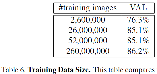
Table 6. Training Data Size. This table compares the performance after 700h of training for a smaller model with 96x96 pixel inputs. The model architecture is similar to NN2, but without the 5x5 convolutions in the Inception modules.表6.培训数据大小。 该表比较了较小型号与96x96像素输入的700h训练后的性能。 模型体系结构类似于NN2，但在Inception模块中没有5x5卷积。

Table 6 shows the impact of large amounts of training data. Due to time constraints this evaluation was run on a smaller model; the effect may be even larger on larger models. It is clear that using tens of millions of exemplars results in a clear boost of accuracy on our personal photo test set from section 4.2. Compared to only millions of images the relative reduction in error is 60%. Using another order of magnitude more images (hundreds of millions) still gives a small boost, but the improvement tapers off.表6显示了大量训练数据的影响。 由于时间限制，此评估是在较小的模型上运行的; 在较大型号上效果可能更大。 很明显，使用数千万个样本可以明显提高4.2节中我们个人照片测试集的准确性。 与仅数百万的图像相比，误差的相对减少为60％。 使用另一个数量级的更多图像（数亿）仍然可以提供小幅提升，但改进逐渐减少。

5.6. 在LFW数据集上的表现

We evaluate our model on LFW using the standard protocol for unrestricted, labeled outside data. Nine training splits are used to select the L2-distance threshold. Classification (same or different) is then performed on the tenth test split. The selected optimal threshold is 1.242 for all test splits except split eighth (1.256).我们使用标准协议评估LFW上的模型，用于不受限制的标记外部数据。 九个训练分裂用于选择L2距离阈值。 然后在第十个测试分割上执行分类（相同或不同）。 对于除分裂八分之一（1.256）之外的所有测试分裂，所选择的最佳阈值是1.242。

Our model is evaluated in two modes:我们的模型有两种评估模式：

• Fixed center crop of the LFW provided thumbnail.固定的LFW中心裁剪提供了缩略图。
• A proprietary face detector (similar to Picasa [3]) is run on the provided LFW thumbnails. If it fails to align the face (this happens for two images), the LFW alignment is used.专有的人脸检测器（类似于Picasa [3]）在提供的LFW缩略图上运行。 如果它无法对齐面部（两个图像会发生这种情况），则使用LFW对齐。

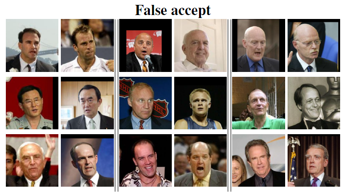
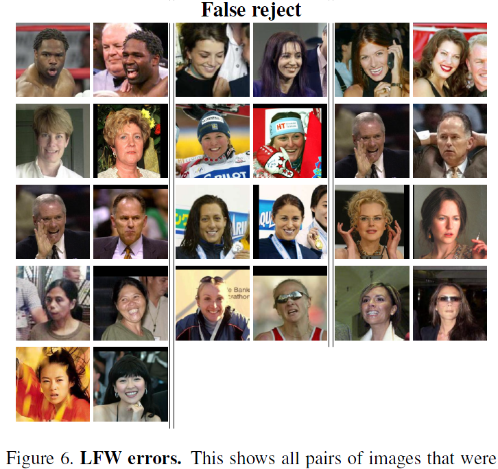
Figure 6. LFW errors. This shows all pairs of images that were incorrectly classified on LFW. Only eight of the 13 false rejects shown here are actual errors the other five are mislabeled in LFW.图6. LFW错误。 这显示了在LFW上错误分类的所有图像对。 这里显示的13个拒绝错误中只有8个是实际错误，其他5个是LFW中的错误标记。

Figure 6 gives an overview of all failure cases. It shows false accepts on the top as well as false rejects at the bottom. We achieve a classification accuracy of 98.87%0:15 when using the fixed center crop described in (1) and the record breaking 99.63%0.09 standard error of the mean when using the extra face alignment (2). This reduces the error reported for DeepFace in [17] by more than a factor of 7 and the previous state-of-the-art reported for DeepId2+ in [15] by 30%. This is the performance of model NN1, but even the much smaller NN3 achieves performance that is not statistically significantly different.图6概述了所有故障情况。 它显示顶部的错误接受以及底部的错误拒绝。 当使用（1）中描述的固定中心作物时，我们实现了98.87％≤0.15的分类精度，并且当使用额外面部对齐时（2），平均值达到99.63％？0.09标准误差。 这将[17]中针对DeepFace报告的错误减少了7倍以上，并且[15]中针对DeepId2 +报告的先前最新技术水平降低了30％。 这是NN1型号的性能，但即使是更小的NN3也能实现统计上没有显着差异的性能。

5.7. 在YouTube Faces DB数据集上的表现

We use the average similarity of all pairs of the first one hundred frames that our face detector detects in each video. This gives us a classification accuracy of 95.12%0:39. Using the first one thousand frames results in 95.18%. Compared to [17] 91.4% who also evaluate one hundred frames per video we reduce the error rate by almost half. DeepId2+ [15] achieved 93.2% and our method reduces this error by 30%, comparable to our improvement on LFW.我们使用人脸检测器在每个视频中检测到的前100帧的所有对的平均相似度。 这使我们的分类准确度为95.12％？0.39。 使用前一千帧导致95.18％。 与[17] 91.4％同时评估每个视频100帧的人相比，我们将错误率降低了近一半。 DeepId2 + [15]达到93.2％，我们的方法将此误差减少了30％，与我们对LFW的改进相当。

5.8. 人脸聚类

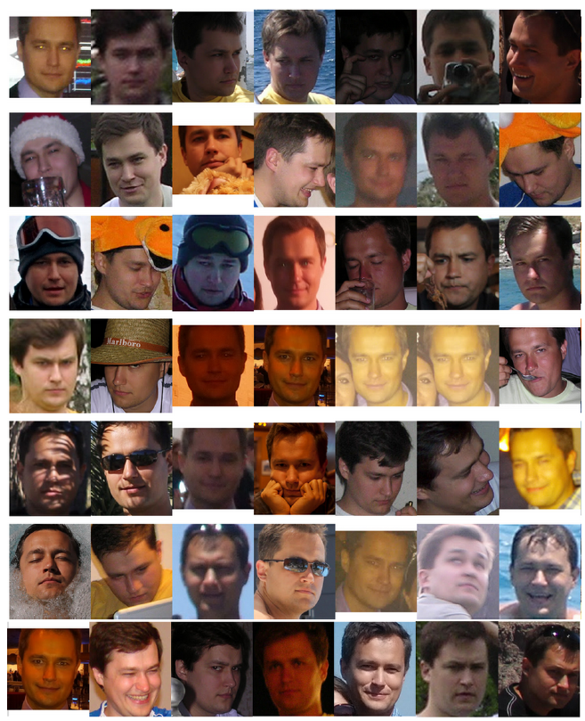
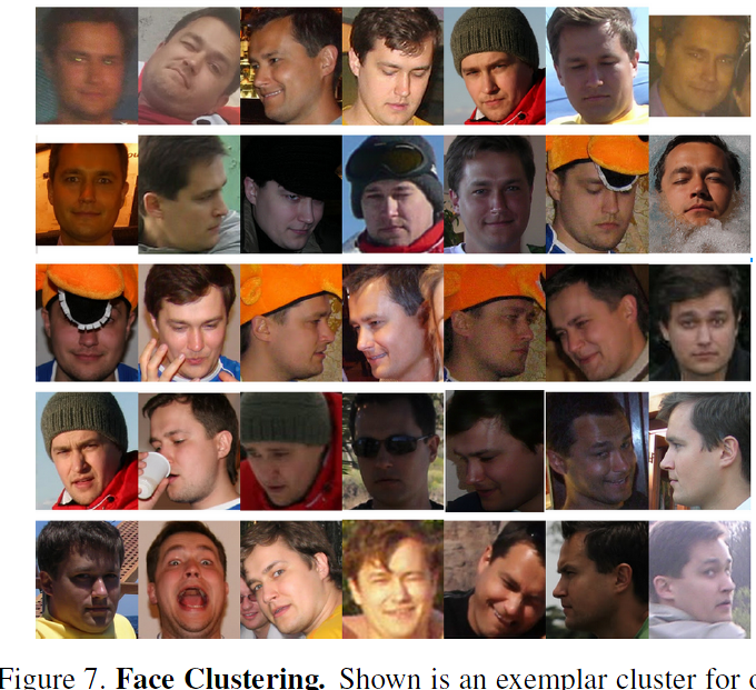
Figure 7. Face Clustering. Shown is an exemplar cluster for one user. All these images in the users personal photo collection were clustered together.图7.面部聚类。 显示的是一个用户的示例群集。 用户个人照片集中的所有这些图像都聚集在一起。

Our compact embedding lends itself to be used in order to cluster a users personal photos into groups of people with the same identity. The constraints in assignment imposed by clustering faces, compared to the pure verification task,lead to truly amazing results. Figure 7 shows one cluster in a users personal photo collection, generated using agglomerative clustering. It is a clear showcase of the incredible invariance to occlusion, lighting, pose and even age.我们的紧凑嵌入适合用于将用户个人照片聚集到具有相同身份的人群中。 与纯验证任务相比，聚类面临的约束导致真正惊人的结果。 图7显示了使用凝聚聚类生成的用户个人照片集中的一个聚类。 它清晰地展示了遮挡，光线，姿势甚至年龄的惊人不变性。

6. 总结

We provide a method to directly learn an embedding into an Euclidean space for face verification. This sets it apart from other methods [15, 17] who use the CNN bottleneck layer, or require additional post-processing such as concatenation of multiple models and PCA, as well as SVM classification. Our end-to-end training both simplifies the setup and shows that directly optimizing a loss relevant to the task at hand improves performance.我们提供了一种直接学习嵌入欧几里德空间进行面部验证的方法。 这使得它与使用CNN瓶颈层的其他方法[15,17]不同，或者需要额外的后处理，例如多个模型和PCA的串联，以及SVM分类。 我们的端到端培训既简化了设置，又表明直接优化与手头任务相关的损失可以提高性能。

Another strength of our model is that it only requires minimal alignment (tight crop around the face area). [17], for example, performs a complex 3D alignment. We also experimented with a similarity transform alignment and notice that this can actually improve performance slightly. It is not clear if it is worth the extra complexity.我们模型的另一个优势是它只需要最小的对齐（面部周围紧密的裁剪）。 [17]，例如，执行复杂的3D对齐。 我们还尝试了相似性变换对齐，并注意到这实际上可以略微提高性能。 目前尚不清楚是否值得额外的复杂性。

Future work will focus on better understanding of the error cases, further improving the model, and also reducing model size and reducing CPU requirements. We will also look into ways of improving the currently extremely long training times, e.g. variations of our curriculum learning with smaller batch sizes and offline as well as online positive and negative mining.未来的工作将侧重于更好地理解错误情况，进一步改进模型，并减少模型大小和降低CPU要求。 我们还将探讨如何改善目前极长的训练时间，例如： 我们的课程学习的变化与较小的批量和离线以及在线积极和消极的挖掘。

7. 附录：谐波嵌入

In this section we introduce the concept of harmonic embeddings. By this we denote a set of embeddings that are generated by different models v1 and v2 but are compatible in the sense that they can be compared to each other.在本节中，我们将介绍谐波嵌入的概念。 通过这个，我们表示由不同模型v1和v2生成的一组嵌入，但是在它们可以彼此比较的意义上是兼容的。

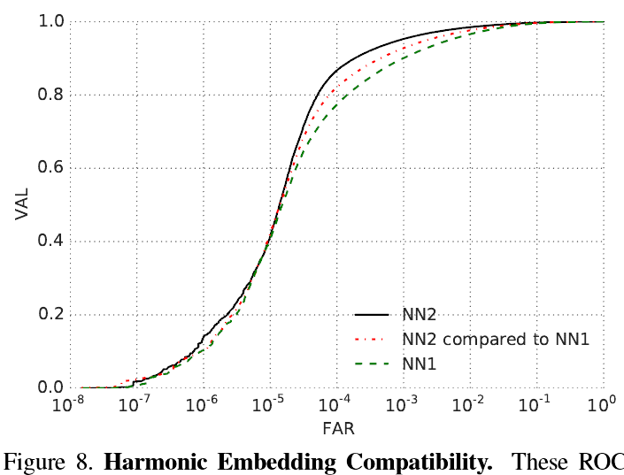
Figure 8. Harmonic Embedding Compatibility. These ROCs show the compatibility of the harmonic embeddings of NN2 to the embeddings of NN1. NN2 is an improved model that performs much better than NN1. When comparing embeddings generated by NN1 to the harmonic ones generated by NN2 we can see the compatibility between the two. In fact, the mixed mode performance is still better than NN1 by itself.图8.谐波嵌入兼容性。 这些ROC显示了NN2的谐波嵌入与NN1嵌入的兼容性。 NN2是一种改进的模型，其性能远优于NN1。 当比较NN1生成的嵌入与NN2生成的谐波嵌入时，我们可以看到两者之间的兼容性。 实际上，混合模式性能本身仍然优于NN1。

This compatibility greatly simplifies upgrade paths. E.g. in an scenario where embedding v1 was computed across a large set of images and a new embedding model v2 is being rolled out, this compatibility ensures a smooth transition without the need to worry about version incompatibilities. Figure 8 shows results on our 3G dataset. It can be seen that the improved model NN2 significantly outperforms NN1, while the comparison of NN2 embeddings to NN1 embeddings performs at an intermediate level.这种兼容性极大地简化了升级路径。 例如。 在一个大型图像集中计算嵌入v1并且正在推出新的嵌入模型v2的情况下，这种兼容性可确保平滑过渡，而无需担心版本不兼容。 图8显示了我们的3G数据集的结果。 可以看出，改进的模型NN2明显优于NN1，而NN2嵌入与NN1嵌入的比较在中间水平上执行。

7.1. 谐波三元组损失

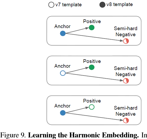
Figure 9. Learning the Harmonic Embedding. In order to learn a harmonic embedding, we generate triplets that mix the v1 embeddings with the v2 embeddings that are being trained. The semihard negatives are selected from the whole set of both v1 and v2 embeddings.图9.学习谐波嵌入。 为了学习谐波嵌入，我们生成三元组，将v1嵌入与正在训练的v2嵌入混合。 从整个v1和v2嵌入集合中选择半硬性负样本。

In order to learn the harmonic embedding we mix embeddings of v1 together with the embeddings v2, that are being learned. This is done inside the triplet loss and results in additionally generated triplets that encourage the compatibility between the different embedding versions. Figure 9 visualizes the different combinations of triplets that contribute to the triplet loss.为了学习谐波嵌入，我们将v1的嵌入与v2的嵌入混合，这是正在学习的。 这是在元组损失内部完成的，并导致额外生成的三元组，这些三元组促进了不同嵌入版本之间的兼容性。 图9显示了导致三重态损失的三重态的不同组合。

We initialized the v2 embedding from an independently trained NN2 and retrained the last layer (embedding layer) from random initialization with the compatibility encouraging triplet loss. First only the last layer is retrained, then we continue training the whole v2 network with the harmonic loss.我们从独立训练的NN2初始化v2嵌入，并从随机初始化中重新训练最后一层（嵌入层），兼容性鼓励三重态丢失。 首先只重新训练最后一层，然后我们继续训练整个v2网络的谐波损失。

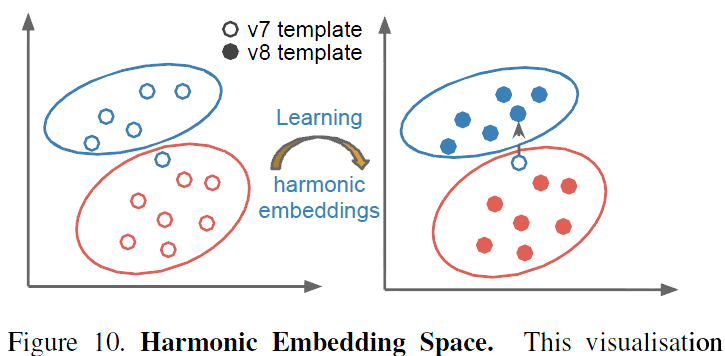
Figure 10. Harmonic Embedding Space. This visualisation sketches a possible interpretation of how harmonic embeddings are able to improve verification accuracy while maintaining compatibility to less accurate embeddings. In this scenario there is one misclassified face, whose embedding is perturbed to the “correct” location in v2.图10.谐波嵌入空间。 该可视化概述了谐波嵌入如何在提高验证准确性的同时保持与不太精确的嵌入的兼容性的可能解释。 在这种情况下，有一个错误分类的面，其嵌入被扰乱到v2中的“正确”位置。

Figure 10 shows a possible interpretation of how this compatibility may work in practice. The vast majority of v2 embeddings may be embedded near the corresponding v1 embedding, however, incorrectly placed v1 embeddings can be perturbed slightly such that their new location in embedding space improves verification accuracy.图10显示了这种兼容性在实践中如何起作用的可能解释。 绝大多数v2嵌入可以嵌入在相应的v1嵌入附近，然而，错误放置的v1嵌入可以稍微扰动，使得它们在嵌入空间中的新位置提高了验证准确性。

7.2. 总结

These are very interesting findings and it is somewhat surprising that it works so well. Future work can explore how far this idea can be extended. Presumably there is a limit as to how much the v2 embedding can improve over v1, while still being compatible. Additionally it would be interesting to train small networks that can run on a mobile phone and are compatible to a larger server side model.这些都是非常有趣的发现，它有点令人惊讶，它运作良好。 未来的工作可以探索这个想法可以扩展到多远。 据推测，v2嵌入可以比v1提高多少，但仍然兼容。 另外，培训可以在移动电话上运行并且与更大的服务器端模型兼容的小型网络将是有趣的。

致谢

We would like to thank Johannes Steffens for his discussions and great insights on face recognition and Christian Szegedy for providing new network architectures like [16] and discussing network design choices. Also we are indebted to the DistBelief [4] team for their support especially to Rajat Monga for help in setting up efficient training schemes.我们要感谢Johannes Steffens关于人脸识别的讨论和深刻见解，以及Christian Szegedy提供的新网络架构，如[16]和讨论网络设计选择。 此外，我们感谢DistBelief [4]团队的支持，尤其是对Rajat Monga的帮助建立有效的培训计划。

Also our work would not have been possible without the support of Chuck Rosenberg, Hartwig Adam, and Simon Han.如果没有Chuck Rosenberg，Hartwig Adam和Simon Han的支持，我们的工作也是不可能的。

参考文献

• [1] Y. Bengio, J. Louradour, R. Collobert, and J. Weston. Curriculum learning. In Proc. of ICML, New York, NY, USA, 2009. 2
• [2] D. Chen, X. Cao, L. Wang, F. Wen, and J. Sun. Bayesian face revisited: A joint formulation. In Proc. ECCV, 2012. 2
• [3] D. Chen, S. Ren, Y. Wei, X. Cao, and J. Sun. Joint cascade face detection and alignment. In Proc. ECCV, 2014. 7
• [4] J. Dean, G. Corrado, R. Monga, K. Chen, M. Devin, M. Mao, M. Ranzato, A. Senior, P. Tucker, K. Yang, Q. V. Le, and A. Y. Ng. Large scale distributed deep networks. In P. Bartlett, F. Pereira, C. Burges, L. Bottou, and K. Weinberger, editors, NIPS, pages 1232–1240. 2012. 10
• [5] J. Duchi, E. Hazan, and Y. Singer. Adaptive subgradient methods for online learning and stochastic optimization. J. Mach. Learn. Res., 12:2121–2159, July 2011. 4
• [6] I. J. Goodfellow, D. Warde-farley, M. Mirza, A. Courville, and Y. Bengio. Maxout networks. In In ICML, 2013. 4
• [7] G. B. Huang, M. Ramesh, T. Berg, and E. Learned-Miller. Labeled faces in the wild: A database for studying face recognition in unconstrained environments. Technical Report 07-49, University of Massachusetts, Amherst, October 2007. 5
• [8] Y. LeCun, B. Boser, J. S. Denker, D. Henderson, R. E. Howard, W. Hubbard, and L. D. Jackel. Backpropagation applied to handwritten zip code recognition. Neural Computation, 1(4):541–551, Dec. 1989. 2, 4
• [9] M. Lin, Q. Chen, and S. Yan. Network in network. CoRR, abs/1312.4400, 2013. 2, 4, 6
• [10] C. Lu and X. Tang. Surpassing human-level face verification performance on LFW with gaussianface. CoRR, abs/1404.3840, 2014. 1
• [11] D. E. Rumelhart, G. E. Hinton, and R. J. Williams. Learning representations by back-propagating errors. Nature, 1986. 2, 4
• [12] M. Schultz and T. Joachims. Learning a distance metric from relative comparisons. In S. Thrun, L. Saul, and B. Schölkopf, editors, NIPS, pages 41–48. MIT Press, 2004. 2
• [13] T. Sim, S. Baker, and M. Bsat. The CMU pose, illumination, and expression (PIE) database. In In Proc. FG, 2002. 2
• [14] Y. Sun, X. Wang, and X. Tang. Deep learning face representation by joint identification-verification. CoRR, abs/1406.4773, 2014. 1, 2, 3
• [15] Y. Sun, X. Wang, and X. Tang. Deeply learned face representations are sparse, selective, and robust. CoRR, abs/1412.1265, 2014. 1, 2, 5, 8
• [16] C. Szegedy, W. Liu, Y. Jia, P. Sermanet, S. Reed, D. Anguelov, D. Erhan, V. Vanhoucke, and A. Rabinovich. Going deeper with convolutions. CoRR, abs/1409.4842, 2014. 2, 3, 4, 5, 6, 10
• [17] Y. Taigman, M. Yang, M. Ranzato, and L. Wolf. Deepface: Closing the gap to human-level performance in face verification. In IEEE Conf. on CVPR, 2014. 1, 2, 5, 7, 8, 9
• [18] J. Wang, Y. Song, T. Leung, C. Rosenberg, J. Wang, J. Philbin, B. Chen, and Y. Wu. Learning fine-grained image similarity with deep ranking. CoRR, abs/1404.4661, 2014. 2
• [19] K. Q.Weinberger, J. Blitzer, and L. K. Saul. Distance metric learning for large margin nearest neighbor classification. In NIPS. MIT Press, 2006. 2, 3
• [20] D. R. Wilson and T. R. Martinez. The general inefficiency of batch training for gradient descent learning. Neural Networks, 16(10):1429–1451, 2003. 4
• [21] L. Wolf, T. Hassner, and I. Maoz. Face recognition in unconstrained videos with matched background similarity. In IEEE Conf. on CVPR, 2011. 5
• [22] M. D. Zeiler and R. Fergus. Visualizing and understanding convolutional networks. CoRR, abs/1311.2901, 2013. 2, 3, 4, 6
• [23] Z. Zhu, P. Luo, X. Wang, and X. Tang. Recover canonicalview faces in the wild with deep neural networks. CoRR, abs/1404.3543, 2014. 2