1、神经网络概述:


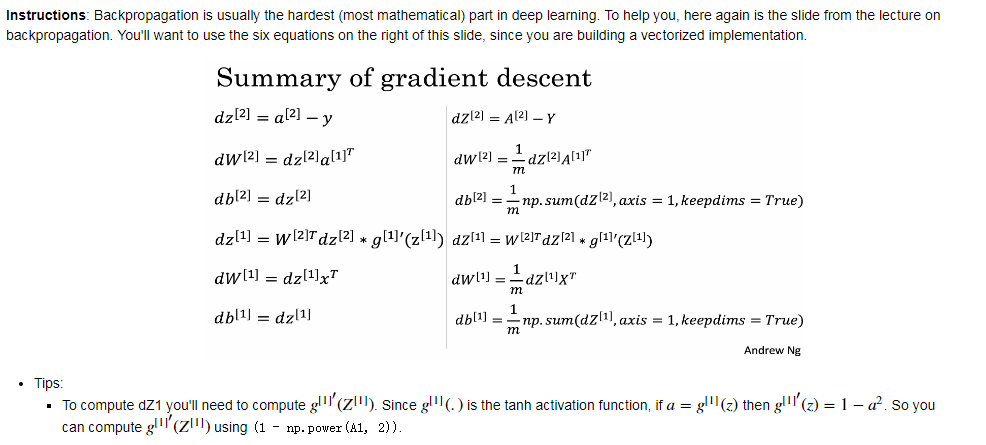
dW[L]=(1/m)*dZ[L]A[L-1].T
db[L]=(1/m)*np.sum(dZ[L],axis=1,keepdims=True)
dZ[L-1]=W[L].T dZ[L]*g'(Z[L-1])
2. 激活函数:
sigmoid(z)=1/(1+e-z), tanh(z)=(ez+e-z)/(ez-e-z) , RelU(z)=max(0,z) , Leaky RelU(z)=max(0.01z,z)
sigmoid(z)'=a(1-a), tanh(z)'=1-a2 , RelU(z)'=1 or 0 , Leaky RelU(z)'=1 or 0.01

sigmoid激活函数:除了输出层是一个二分类问题基本不会用它;
tanh激活函数:tanh是非常优秀的,几乎适合所有场合;
ReLu激活函数:最常用的默认函数,如果不确定用哪个激活函数,就使用ReLu或者Leaky ReLu;
3.随机初始化:
W[L]=np.random.randn(nL,nL-1)*0.01
bL=np.zeros((nL,1)
4.编程实践:


  1 #Defining the neural network structure:
  2 def layer_sizes(X, Y):
  3     """
  4     Arguments:
  5     X -- input dataset of shape (input size, number of examples)
  6     Y -- labels of shape (output size, number of examples)
  7
  8     Returns:
  9     n_x -- the size of the input layer
 10     n_h -- the size of the hidden layer
 11     n_y -- the size of the output layer
 12     """
 13     n_x = X.shape[0] # size of input layer
 14     n_h = 4
 15     n_y =X.shape[0] # size of output layer
 16
 17     return (n_x, n_h, n_y)
 18
 19 #Initialize the model's parameters
 20 def initialize_parameters(n_x, n_h, n_y):
 21     """
 22     Argument:
 23     n_x -- size of the input layer
 24     n_h -- size of the hidden layer
 25     n_y -- size of the output layer
 26
 27     Returns:
 28     params -- python dictionary containing your parameters:
 29                     W1 -- weight matrix of shape (n_h, n_x)
 30                     b1 -- bias vector of shape (n_h, 1)
 31                     W2 -- weight matrix of shape (n_y, n_h)
 32                     b2 -- bias vector of shape (n_y, 1)
 33     """
 34
 35     np.random.seed(2) # we set up a seed so that your output matches ours although the initialization is random.
 36
 37     ### START CODE HERE ### (≈ 4 lines of code)
 38     W1 = np.random.randn(n_h,n_x)*0.01
 39     b1 = np.zeros((n_h,1))
 40     W2 = np.random.randn(n_y,n_h)*0.01
 41     b2 = np.zeros((n_y,0))
 42
 43     ### END CODE HERE ###
 44
 45     assert (W1.shape == (n_h, n_x))
 46     assert (b1.shape == (n_h, 1))
 47     assert (W2.shape == (n_y, n_h))
 48     assert (b2.shape == (n_y, 1))
 49
 50     parameters = {"W1": W1,
 51                   "b1": b1,
 52                   "W2": W2,
 53                   "b2": b2}
 54
 55     return parameters
 56
 57 #Implement forward_propagation()
 58 def forward_propagation(X, parameters):
 59     """
 60     Argument:
 61     X -- input data of size (n_x, m)
 62     parameters -- python dictionary containing your parameters (output of initialization function)
 63
 64     Returns:
 65     A2 -- The sigmoid output of the second activation
 66     cache -- a dictionary containing "Z1", "A1", "Z2" and "A2"
 67     """
 68     # Retrieve each parameter from the dictionary "parameters"
 69     ### START CODE HERE ### (≈ 4 lines of code)
 70     W1 = parameters['W1']
 71     b1 = parameters['b1']
 72     W2 = parameters['W2']
 73     b2 = parameters['b2']
 74     ### END CODE HERE ###
 75
 76     # Implement Forward Propagation to calculate A2 (probabilities)
 77     ### START CODE HERE ### (≈ 4 lines of code)
 78     Z1 = np.dot(W1,X)+b1
 79     A1 = np.tanh(Z1)
 80     Z2 = np.dot(W2,A1)+b2
 81     A2 = sigmoid(Z2)
 82     ### END CODE HERE ###
 83
 84     assert(A2.shape == (1, X.shape[1]))
 85
 86     cache = {"Z1": Z1,
 87              "A1": A1,
 88              "Z2": Z2,
 89              "A2": A2}
 90
 91     return A2, cache
 92
 93 #implement  compute_cost
 94 def compute_cost(A2, Y, parameters):
 95     """
 96     Computes the cross-entropy cost given in equation (13)
 97
 98     Arguments:
 99     A2 -- The sigmoid output of the second activation, of shape (1, number of examples)
100     Y -- "true" labels vector of shape (1, number of examples)
101     parameters -- python dictionary containing your parameters W1, b1, W2 and b2
102
103     Returns:
104     cost -- cross-entropy cost given equation (13)
105     """
106
107     m = Y.shape[1] # number of example
108
109     # Compute the cross-entropy cost
110     ### START CODE HERE ### (≈ 2 lines of code)
111     logprobs = np.multiply(np.log(A2),Y)+np.multiply((1-Y),np.log((1-A2)))
112     cost =np.sum(logprobs)/m
113     ### END CODE HERE ###
114
115     cost = np.squeeze(cost)     # makes sure cost is the dimension we expect.
116                                 # E.g., turns [[17]] into 17
117     assert(isinstance(cost, float))
118
119     return cost
120
121 #implement backward_propagation:
122 def backward_propagation(parameters, cache, X, Y):
123     """
124     Implement the backward propagation using the instructions above.
125
126     Arguments:
127     parameters -- python dictionary containing our parameters
128     cache -- a dictionary containing "Z1", "A1", "Z2" and "A2".
129     X -- input data of shape (2, number of examples)
130     Y -- "true" labels vector of shape (1, number of examples)
131
132     Returns:
133     grads -- python dictionary containing your gradients with respect to different parameters
134     """
135     m = X.shape[1]
136
137     # First, retrieve W1 and W2 from the dictionary "parameters".
138     ### START CODE HERE ### (≈ 2 lines of code)
139     W1 = parameters['W1']
140     W2 = parameters['W2']
141     ### END CODE HERE ###
142
143     # Retrieve also A1 and A2 from dictionary "cache".
144     ### START CODE HERE ### (≈ 2 lines of code)
145     A1 = cache['A1']
146     A2 = cache['A2']
147     ### END CODE HERE ###
148
149     # Backward propagation: calculate dW1, db1, dW2, db2.
150     ### START CODE HERE ### (≈ 6 lines of code, corresponding to 6 equations on slide above)
151     dZ2 = A2-Y
152     dW2 = (1.0/m)*np.dot(dZ2,A1.T)
153     db2 = (1.0/m)*np.sum(dZ2,axis=1,keepdims=True)
154     dZ1 = np.multiply(np.dot(W2.T,dZ2),(1-np.power(A1,2)))
155     dW1 = (1.0/m)*np.dot(dZ1,X.T)
156     db1 = (1.0/m)*np.sum(dZ1,axis=1,keepdims=True)
157     ### END CODE HERE ###
158
159     grads = {"dW1": dW1,
160              "db1": db1,
161              "dW2": dW2,
162              "db2": db2}
163
164     return grads
165
166 #update_parameters:
167 def update_parameters(parameters, grads, learning_rate = 1.2):
168     """
169     Updates parameters using the gradient descent update rule given above
170
171     Arguments:
172     parameters -- python dictionary containing your parameters
173     grads -- python dictionary containing your gradients
174
175     Returns:
176     parameters -- python dictionary containing your updated parameters
177     """
178     # Retrieve each parameter from the dictionary "parameters"
179     ### START CODE HERE ### (≈ 4 lines of code)
180     W1 = parameters['W1']
181     b1 = parameters['b1']
182     W2 = parameters['W2']
183     b2 = parameters['b2']
184     ### END CODE HERE ###
185
186     # Retrieve each gradient from the dictionary "grads"
187     ### START CODE HERE ### (≈ 4 lines of code)
188     dW1 = grads['dW1']
189     db1 = grads['db1']
190     dW2 = grads['dW2']
191     db2 = grads['db2']
192     ## END CODE HERE ###
193
194     # Update rule for each parameter
195     ### START CODE HERE ### (≈ 4 lines of code)
196     W1 = W1-learning_rate*dW1
197     b1 = b1-learning_rate*db1
198     W2 = W2-learning_rate*dW2
199     b2 = b2-learning_rate*db2
200     ### END CODE HERE ###
201
202     parameters = {"W1": W1,
203                   "b1": b1,
204                   "W2": W2,
205                   "b2": b2}
206
207     return parameters
208
209 #Build your neural network model
210 def nn_model(X, Y, n_h, num_iterations = 10000, print_cost=False):
211     """
212     Arguments:
213     X -- dataset of shape (2, number of examples)
214     Y -- labels of shape (1, number of examples)
215     n_h -- size of the hidden layer
216     num_iterations -- Number of iterations in gradient descent loop
217     print_cost -- if True, print the cost every 1000 iterations
218
219     Returns:
220     parameters -- parameters learnt by the model. They can then be used to predict.
221     """
222
223     np.random.seed(3)
224     n_x = layer_sizes(X, Y)[0]
225     n_y = layer_sizes(X, Y)[2]
226
227     # Initialize parameters, then retrieve W1, b1, W2, b2. Inputs: "n_x, n_h, n_y". Outputs = "W1, b1, W2, b2, parameters".
228     ### START CODE HERE ### (≈ 5 lines of code)
229     parameters = initialize_parameters(n_x,n_h,n_y)
230     W1 = parameters['W1']
231     b1 = parameters['b1']
232     W2 = parameters['W2']
233     b2 = parameters['b2']
234     ### END CODE HERE ###
235
236     # Loop (gradient descent)
237
238     for i in range(0, num_iterations):
239
240         ### START CODE HERE ### (≈ 4 lines of code)
241         # Forward propagation. Inputs: "X, parameters". Outputs: "A2, cache".
242         A2, cache = forward_propagation(X,parameters)
243
244         # Cost function. Inputs: "A2, Y, parameters". Outputs: "cost".
245         cost =compute_cost(A2,Y,parameters)
246
247         # Backpropagation. Inputs: "parameters, cache, X, Y". Outputs: "grads".
248         grads =backward_propagation(parameters,cache,X,Y)
249
250         # Gradient descent parameter update. Inputs: "parameters, grads". Outputs: "parameters".
251         parameters = update_parameters(parameters,grads)
252
253         ### END CODE HERE ###
254
255         # Print the cost every 1000 iterations
256         if print_cost and i % 1000 == 0:
257             print ("Cost after iteration %i: %f" %(i, cost))
258
259     return parameters
260
261 #Use your model to predict by building predict().Use forward propagation to predict results
262
263 def predict(parameters, X):
264     """
265     Using the learned parameters, predicts a class for each example in X
266
267     Arguments:
268     parameters -- python dictionary containing your parameters
269     X -- input data of size (n_x, m)
270
271     Returns
272     predictions -- vector of predictions of our model (red: 0 / blue: 1)
273     """
274
275     # Computes probabilities using forward propagation, and classifies to 0/1 using 0.5 as the threshold.
276     ### START CODE HERE ### (≈ 2 lines of code)
277     A2, cache = forward_propagation(X,parameters)
278     predictions =np.where(A2>0.5,1,0)
279     ### END CODE HERE ###
280
281     return predictions