朴素贝叶斯算法应用——垃圾短信分类

理解贝叶斯公式其实就只要掌握：1、条件概率的定义；2、乘法原理

$P(c_i|x) = \cfrac{P(x|c_i)P(c_i)}{P(x)}$

这里 $x$ 是一个向量，有几个特征，就有几个维度。朴素贝叶斯就假设这些特征独立同分布，即

$P(x|c_i) = P(x_1|c_i)P(x_2|c_i) \cdots P(x_n|c_i)$

在实现朴素贝叶斯的时候，还要注意一写技巧：

1、数据平滑处理；
2、在计算机中，多个小数相乘趋于 0 ，因此，常常对每一个概率取对数（这种情况很多书籍上称之为“下溢”）。

数据下载：http://archive.ics.uci.edu/ml/datasets.html

关于短信的分类在这个网页下载：http://archive.ics.uci.edu/ml/datasets/SMS+Spam+Collection

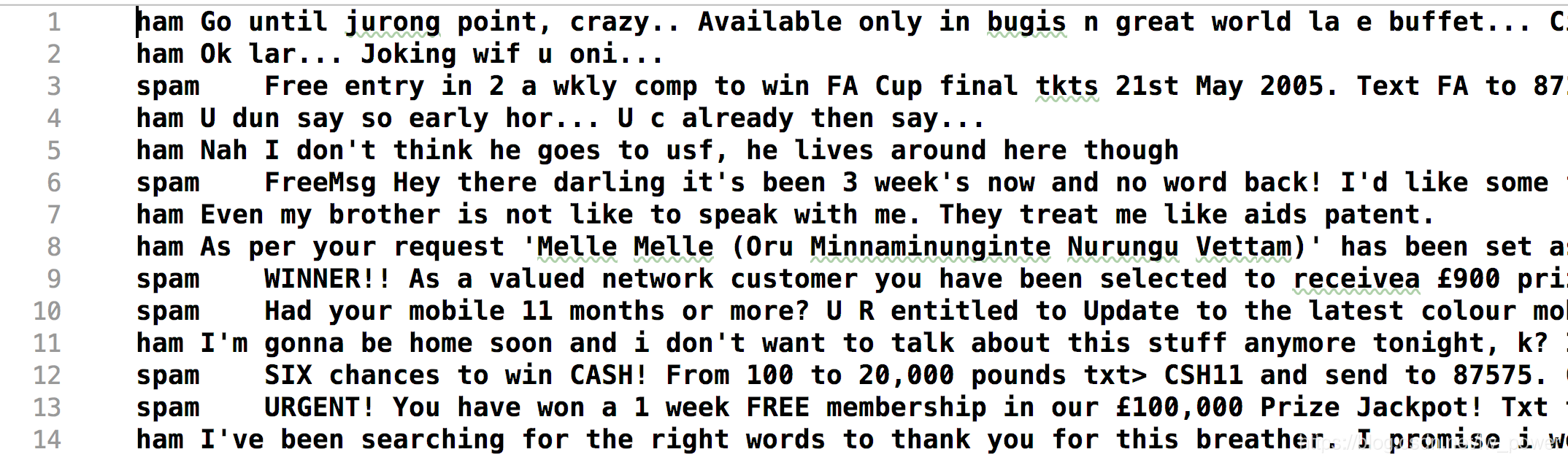
数据如下：每一行表示一条信息和真实的分类结果。一行的开始不是 ham 就是 spam，其中，ham 表示合理合法的邮件，spam 表示是一些广告，即垃圾短信。

在这里插入图片描述

数据预处理

每一行按照分隔符 “\t” 分割成前后两部分：
第 1 部分：标识短信是否是垃圾短信；
第 2 部分：一条短信的具体内容。

第 2 部分还要继续做处理：
1、按照空格进行分割，即分词，如果是中文短信，就要使用一些中文分词库了；
2、把分割以后的单词全部处理成小写；
语法上的大小写不应该被算法认为是两个词。
3、去除停用词：
这一步，实际上就是把一些常见的词“你”、“我”、“他”、“是”、“的”之内的去掉，这些词很大很长度上也只是撑起了句子的结构，对表达句子的情感来说，没有帮助。

我们的做法比较粗暴，把长度小于 3 的单词全部去掉了。

参考代码：

class FileOperate:

    def __init__(self, data_path, label):
        self.data_path = data_path
        self.label = label

    def load_data(self):
        with open(self.data_path, 'r', encoding='utf-8') as fr:
            content = fr.readlines()
            print("一共 {} 条数据。".format(len(content)))

        X = list()
        y = list()

        for line in content:
            result = line.split(self.label, maxsplit=2)
            X.append(FileOperate.__clean_data(result[1]))
            y.append(1 if result[0]=='spam' else 0)

        return X, y

    @staticmethod
    def __clean_data(origin_info):
        '''
        清洗数据，去掉非字母的字符，和字节长度小于 2 的单词
        :return:
        '''
        # 先转换成小写
        # 把标点符号都替换成空格
        temp_info = re.sub('\W', ' ', origin_info.lower())
        # 根据空格（大于等于 1 个空格）
        words = re.split(r'\s+', temp_info)
        return list(filter(lambda x: len(x) >= 3, words))

经过上面的处理，得到的一条短信的实际上是下面这样一个单词列表：

['until', 'jurong', 'point', 'crazy', 'available', 'only', 'bugis', 'great', 'world', 'buffet', 'cine', 'there', 'got', 'amore', 'wat']

接下来，把全部的数据集分成训练数据集和测试数据集

开始训练

根据公式

$P(c_i|x) = \cfrac{P(x|c_i)P(c_i)}{P(x)}$

1、首先建立单词表，这个单词表是从所有的数据中得到；
2、然后针对两个类别，分别统计单词表出现的次数，其实就是 word count，用一个 map（Python 中叫 dict）去统计词频；

这里有个细节：

很可能在某个类别中，某个单词不出现，即频数为 0，那么频率也为 0，于是连乘以后积就为 0 ，在这里就要做拉普拉斯平滑。同理，对类别也要做拉普拉斯平滑。

参考代码（包含了预测的代码，看这一部分的时候可以暂时略过，只看 fit 的部分，fit 其实就是在做单词频数统计）：

class NaiveBayes:

    def __init__(self):
        self.__ham_count = 0  # 非垃圾短信数量
        self.__spam_count = 0  # 垃圾短信数量

        self.__ham_words_count = 0  # 非垃圾短信单词总数
        self.__spam_words_count = 0  # 垃圾短信单词总数

        self.__ham_words = list()  # 非垃圾短信单词列表
        self.__spam_words = list()  # 垃圾短信单词列表

        # 训练集中不重复单词集合
        self.__word_dictionary_set = set()

        self.__word_dictionary_size = 0

        self.__ham_map = dict()  # 非垃圾短信的词频统计
        self.__spam_map = dict()  # 垃圾短信的词频统计

        self.__ham_probability = 0
        self.__spam_probability = 0

    def fit(self, X_train, y_train):
        self.build_word_set(X_train, y_train)
        self.word_count()

    def predict(self, X_train):
        return [self.predict_one(sentence) for sentence in X_train]

    def build_word_set(self, X_train, y_train):
        '''
        第 1 步：建立单词集合
        :param X_train:
        :param y_train:
        :return:
        '''
        for words, y in zip(X_train, y_train):
            if y == 0:
                # 非垃圾短信
                self.__ham_count += 1
                self.__ham_words_count += len(words)
                for word in words:
                    self.__ham_words.append(word)
                    self.__word_dictionary_set.add(word)
            if y == 1:
                # 垃圾短信
                self.__spam_count += 1
                self.__spam_words_count += len(words)
                for word in words:
                    self.__spam_words.append(word)
                    self.__word_dictionary_set.add(word)

        # print('非垃圾短信数量', self.__ham_count)
        # print('垃圾短信数量', self.__spam_count)
        # print('非垃圾短信单词总数', self.__ham_words_count)
        # print('垃圾短信单词总数', self.__spam_words_count)
        # print(self.__word_dictionary_set)
        self.__word_dictionary_size = len(self.__word_dictionary_set)

    def word_count(self):
        # 第 2 步：不同类别下的词频统计
        for word in self.__ham_words:
            self.__ham_map[word] = self.__ham_map.setdefault(word, 0) + 1

        for word in self.__spam_words:
            self.__spam_map[word] = self.__spam_map.setdefault(word, 0) + 1

        # 【下面两行计算先验概率】
        # 非垃圾短信的概率
        self.__ham_probability = self.__ham_count / (self.__ham_count + self.__spam_count)
        # 垃圾短信的概率
        self.__spam_probability = self.__spam_count / (self.__ham_count + self.__spam_count)

    def predict_one(self, sentence):
        ham_pro = 0
        spam_pro = 0

        for word in sentence:
            # print('word', word)
            ham_pro += math.log(
                (self.__ham_map.get(word, 0) + 1) / (self.__ham_count + self.__word_dictionary_size))

            spam_pro += math.log(
                (self.__spam_map.get(word, 0) + 1) / (self.__spam_count + self.__word_dictionary_size))

        ham_pro += math.log(self.__ham_probability)
        spam_pro += math.log(self.__spam_probability)

        # print('垃圾短信概率', spam_pro)
        # print('非垃圾短信概率', ham_pro)
        return int(spam_pro >= ham_pro)

预测

我们再看看朴素贝叶斯公式：

$P(c_i|x) = \cfrac{P(x|c_i)P(c_i)}{P(x)} = \cfrac{P(x_1|c_i)P(x_2|c_i) \cdots P(x_n|c_i) \cdot P(c_i)}{P(x)}$

对于一条预测数据，分别针对两个类，计算分子的对数，然后比较大小即可，即

朴素贝叶斯其实就是这么简单。在这个数据集上，我们可以得到准确率：0.9755922469490309。

（把代码传到 GitHub 上。）

我们这个例子只是对于二分类问题而言，并且特征都是离散型的。朴素贝叶斯在 scikit-learn 上有伯努利朴素贝叶斯（就是我们这个例子使用到的模型），多项式朴素贝叶斯、高斯朴素贝叶斯，这些在刘建平的文章《scikit-learn 朴素贝叶斯类库使用小结》（https://www.cnblogs.com/pinard/p/6074222.html）中有介绍。

参考资料

1、李航《统计学习方法》
关键词：贝叶斯估计、拉普拉斯平滑
2、周志华《机器学习》
这两本教材上都给出了详细的讲解和例子。
3、《机器学习实战》
这本书上给出了参考的代码，但是代码比较冗长，看起来会有点累。

其它在网络上的参考资料：

朴素贝叶斯分类器详解及中文文本舆情分析（附代码实践）
https://mp.weixin.qq.com/s/Pi30jA1xUbXg3dSdlvdU-g

深入理解朴素贝叶斯（Naive Bayes）
https://blog.csdn.net/li8zi8fa/article/details/76176597

刘建平：朴素贝叶斯算法原理小结
https://www.cnblogs.com/pinard/p/6069267.html