图像风格迁移——《A Neural Algorithm of Artistic Style》

之前看到别人玩图像风格迁移，感觉挺有意思的，趁着空下来的时间自己玩了一下。还是沿着老方法，先看一下论文，然后跑跑程序。论文看的是最基础的《A Neural Algorithm of Artistic Style》，程序嘛，当然不是笨妞自己写的，跑了keras安装文件夹下examples里面的例子

1. 论文概括

这篇论文写得很容易懂，虽然连笨妞这么啰嗦的人都觉得有点啰嗦。原本想直接翻译的，但是，实际核心内容并不多，就直接概括一下吧。

作者的目的是想把艺术大师的名画的画风迁移到普通的图片上，使机器也可以画名画。这就涉及到两方面的图片——画风图片（一般是名画）、内容图片（我们想画的内容）。

具体实现的方式用框图表示出来是这样的

实际操作是通过不带全连接层的vgg网络分别抽取内容图、画风图以及生成图（就是最后你画的“名画”）的特征图，然后分别用内容特征和生成特征图计算内容损失，用画风图和生成图计算风格损失，将两个损失合起来，作为总体损失，用总体损失来计算生成图的梯度然后更新生成图。生成图最初初始化为白噪声图。vgg用imagenet预训练模型。

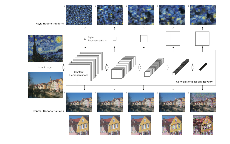
作者的意图是想通过CNN分别抽取内容图的特征图、名画的特征图。然后用内容特征图做出目标内容；用画风特征图做出目标画风。根据生成图的内容与目标内容的差异来“画”（优化）内容；用生成图与目标画风的差异来“画”（优化）风格。（下面这句为个人理解）这样一来，上面框图中最上面的网络和最下面的网络实际只跑一次，但中间网络要跑N次，但这N次跑前向和后向，后向不会优化网络参数，只会优化生成图。

特征图可以选择vgg 5个卷积模块中任何一个模块的仁义卷积层的输出，实际画风提取了多个卷积层的输出。内容直接用特征图表示；画风采用每个特征图自己与自己的格拉姆矩阵表示，通常将多个卷积层提取的多个特征图作格拉姆矩阵后叠加。

格拉姆矩阵是计算相关关系的，个人以为计算特征图自己的格拉姆矩阵是提取像素与像素之间的关联，以这种关联性来表示风格。

论文中实际方法是这样的：

内容的损失和基于生成图的梯度

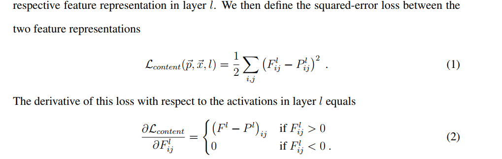
其中Fij和Pij分别表示生成图像和原始内容图像中的像素值。

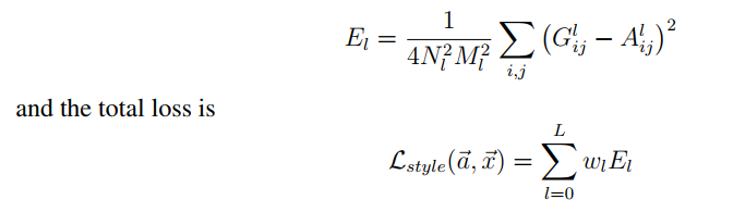
画风损失和基于生成图的梯度

画风损失——名画的格拉姆矩阵和要生成图的格拉姆矩阵之间的距离总和

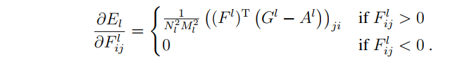
画风基于生成图的梯度

总损失

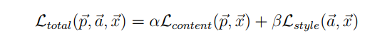
以总损失作为目标优化生成图。

2. 实际操练

实际操作过程中，可以分成以下几步：

A. 图像预处理(内容图、画风图）、生成图占位符定义

B. 预训练模型加载

C. 三张图跑网络

D. 内容损失计算

E.格拉姆矩阵计算

F. 风格损失计算

G. 损失和梯度汇总

H. 设置迭代计算图

I.选择生成图优化方法

J. 开始迭代

程序如下：

from __future__ import print_function
from keras.preprocessing.image import load_img, img_to_array
from scipy.misc import imsave
import numpy as np
from scipy.optimize import fmin_l_bfgs_b
import time
import argparse

from keras.applications import vgg19
from keras import backend as K

import sys

#解析参数的定义和添加
paser = parser = argparse.ArgumentParser(description='Neural style transfer with Keras.')
parser.add_argument('--base_image_path',  type=str, default='image/boy1.jpg', required=False,
                    help='Path to the image to transform.')
parser.add_argument('--style_reference_image_path', default='image/style/style_6.jpg', type=str, required=False,
                    help='Path to the style reference image.')
parser.add_argument('--result_prefix', default='boy_style_transfer', type=str, required=False,
                    help='Prefix for the saved results.')
parser.add_argument('--iter', type=int, default=10, required=False,
                    help='Number of iterations to run.')
parser.add_argument('--content_weight', type=float, default=0.025, required=False,
                    help='Content weight.')
parser.add_argument('--style_weight', type=float, default=1.0, required=False,
                    help='Style weight.')
parser.add_argument('--tv_weight', type=float, default=1.0, required=False,
                    help='Total Variation weight.')

#自定义参数的设置
args = parser.parse_args(['--base_image_path', 'image/spring.jpg'])
#args = parser.parse_args()
base_image_path = args.base_image_path
style_reference_image_path = args.style_reference_image_path
result_prefix = args.result_prefix
iterations = args.iter

# these are the weights of the different loss components
total_variation_weight = args.tv_weight
style_weight = args.style_weight
content_weight = args.content_weight

# dimensions of the generated picture.
width, height = load_img(base_image_path).size
img_nrows = 400
img_ncols = int(width * img_nrows / height)

#图像预处理
def preprocess_image(image_path):
    #读入图像，并转化为目标尺寸。
    img = load_img(image_path, target_size=(img_nrows, img_ncols))
    img = img_to_array(img)
    img = np.expand_dims(img, axis=0) #3
    #vgg提供的预处理，主要完成（1）去均值（2）RGB转BGR（3）维度调换三个任务。
    img = vgg19.preprocess_input(img)
    return img

#图像后处理
def deprocess_image(x):
    if K.image_dim_ordering() == 'th':
        x = x.reshape((3, img_nrows, img_ncols))
        x = x.transpose((1, 2, 0))
    else:
        x = x.reshape((img_nrows, img_ncols, 3))
   
    x[:, :, 0] += 103.939
    x[:, :, 1] += 116.779
    x[:, :, 2] += 123.68
    # 'BGR'->'RGB'
    x = x[:, :, ::-1]
    x = np.clip(x, 0, 255).astype('uint8')
    return x


#读入内容图和风格图，预处理，并包装成变量。这里把内容图和风格图都做成尺寸相同的了，有点不灵活。
base_image = K.variable(preprocess_image(base_image_path))
style_reference_image = K.variable(preprocess_image(style_reference_image_path))

#给目标图片定义占位符，目标图像与resize后的内容图大小相同。
if K.image_dim_ordering() == 'th':
    combination_image = K.placeholder((1, 3, img_nrows, img_ncols))
else:
    combination_image = K.placeholder((1, img_nrows, img_ncols, 3))

#将三个张量串联到一起，形成一个形如（3,3,img_nrows,img_ncols）的张量
#三张图一同喂入网络中，以batch的形式
input_tensor = K.concatenate([base_image, style_reference_image, combination_image], axis=0)

#加载vgg19预训练模型，模型由imagenet预训练。去掉模型的全连接层。
model = vgg19.VGG19(input_tensor=input_tensor,
                    weights='imagenet', include_top=False)
print('Model loaded.')

# get the symbolic outputs of each "key" layer (we gave them unique names).
outputs_dict = dict([(layer.name, layer.output) for layer in model.layers])

#计算特征图的格拉姆矩阵，格拉姆矩阵算两者的相关性，这里算的是一张特征图的自相关。
#个人理解为是像素或者区域间的相关性。用这个相关性来代表风格是的表示。
def gram_matrix(x):
    assert K.ndim(x) == 3
    if K.image_data_format() == 'channels_first':
        features = K.batch_flatten(x)
    else:
        features = K.batch_flatten(K.permute_dimensions(x, (2, 0, 1)))
    gram = K.dot(features, K.transpose(features))
    return gram

#计算风格图的格拉姆矩阵
#计算生成图的格拉姆矩阵
#计算风格图与生成图之间的格拉姆矩阵的距离，作为风格loss
def style_loss(style, combination):
    assert K.ndim(style) == 3
    assert K.ndim(combination) == 3
    S = gram_matrix(style)
    C = gram_matrix(combination)
    channels = 3
    size = img_nrows * img_ncols
    return K.sum(K.square(S - C)) / (4. * (channels ** 2) * (size ** 2))

#内容图和生成图之间的距离作为内容loss
def content_loss(base, combination):
    return K.sum(K.square(combination - base))

#计算变异loss(不太明白)
def total_variation_loss(x):
    assert K.ndim(x) == 4
    if K.image_data_format() == 'channels_first':
        a = K.square(x[:, :, :img_nrows - 1, :img_ncols - 1] - x[:, :, 1:, :img_ncols - 1])
        b = K.square(x[:, :, :img_nrows - 1, :img_ncols - 1] - x[:, :, :img_nrows - 1, 1:])
    else:
        a = K.square(x[:, :img_nrows - 1, :img_ncols - 1, :] - x[:, 1:, :img_ncols - 1, :])
        b = K.square(x[:, :img_nrows - 1, :img_ncols - 1, :] - x[:, :img_nrows - 1, 1:, :])
    return K.sum(K.pow(a + b, 1.25))

#以第5卷积块第2个卷积层的特征图为输出。
loss = K.variable(0.)
layer_features = outputs_dict['block5_conv2']
#抽取内容特征图和生成特征图
base_image_features = layer_features[0, :, :, :]
combination_features = layer_features[2, :, :, :]
#计算内容loss
loss += content_weight * content_loss(base_image_features,
                                      combination_features)

feature_layers = ['block1_conv1', 'block2_conv1',
                  'block3_conv1', 'block4_conv1',
                  'block5_conv1']
#抽取风格图和生成图每个卷积块第一个卷积层输出的特征图
#并逐层计算风格loss，叠加在到loss中
for layer_name in feature_layers:
    layer_features = outputs_dict[layer_name]
    style_reference_features = layer_features[1, :, :, :]
    combination_features = layer_features[2, :, :, :]
    sl = style_loss(style_reference_features, combination_features)
    loss += (style_weight / len(feature_layers)) * sl
#叠加生成图像的变异loss
loss += total_variation_weight * total_variation_loss(combination_image)

# 计算生成图像的梯度
grads = K.gradients(loss, combination_image)

#output[0]为loss，剩下的是grad
outputs = [loss]
if isinstance(grads, (list, tuple)):
    outputs += grads
else:
    outputs.append(grads)
#定义需要迭代优化过程的计算图。
#前面三张图一起跑了一次网络只是抽取特征而已，而这里定义了真正训练过程的计算图。
#计算图的前向传导以生成图为输入，以loss和grad为输出，反过来就是优化过程。
#在初始化之前，生成图仍然只是占位符而已。
f_outputs = K.function([combination_image], outputs)

#同时取出loss和grad
def eval_loss_and_grads(x):
    if K.image_data_format() == 'channels_first':
        x = x.reshape((1, 3, img_nrows, img_ncols))
    else:
        x = x.reshape((1, img_nrows, img_ncols, 3))
    outs = f_outputs([x])
    loss_value = outs[0]
    if len(outs[1:]) == 1:
        grad_values = outs[1].flatten().astype('float64')
    else:
        grad_values = np.array(outs[1:]).flatten().astype('float64')
    return loss_value, grad_values

#这个类在前面同时计算出loss和grad的基础上，通过不同的函数分别获取loss和grad。
#原因在于scipy优化函数通过不同的函数获取loss和grad。
class Evaluator(object):

    def __init__(self):
        self.loss_value = None
        self.grads_values = None

    def loss(self, x):
        assert self.loss_value is None
        loss_value, grad_values = eval_loss_and_grads(x)
        self.loss_value = loss_value
        self.grad_values = grad_values
        return self.loss_value

    def grads(self, x):
        assert self.loss_value is not None
        grad_values = np.copy(self.grad_values)
        self.loss_value = None
        self.grad_values = None
        return grad_values

evaluator = Evaluator()

# run scipy-based optimization (L-BFGS) over the pixels of the generated image
# so as to minimize the neural style loss
#x的初始化，初始化成内容图
#为什么不是论文中的白噪声图呢？不解。
x = preprocess_image(base_image_path)

#迭代优化过程
for i in range(iterations):
    print('Start of iteration', i)
    start_time = time.time()
    #使用L-BFGS-B算法优化
    #不断被优化的是x，也就是生成图。
    x, min_val, info = fmin_l_bfgs_b(evaluator.loss, x.flatten(),
                                     fprime=evaluator.grads, maxfun=20)
    print('Current loss value:', min_val)
    # save current generated image
    #图像后处理
    img = deprocess_image(x.copy())
    #保存图像
    fname = result_prefix + '_at_iteration_%d.png' % i
    imsave(fname, img)
    end_time = time.time()
    print('Image saved as', fname)
    print('Iteration %d completed in %ds' % (i, end_time - start_time))

3. 效果

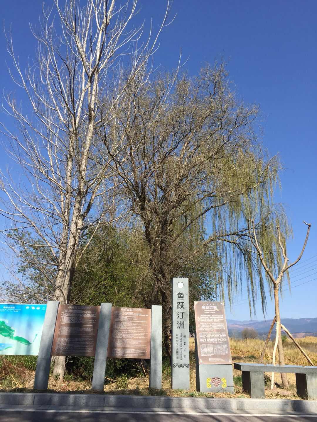
内容图

名画

生成图，经过10次迭代后的结果

4. 个人感想

说实话，笨妞并不觉得这个“画”得好，也不觉得意义有多大（也可能是我迭代次数太少，或者使用的方法太低级）。

笨妞使用的这个模型有一个很大的弊端：内容图和画风图的尺寸和目标图尺寸不能相差太远，尤其是不能太小，不然出来的效果图会有模糊感。