Sequence Models
This is the fifth and final course of the deep learning specialization at Coursera which is moderated by deeplearning.ai
Here are the course summary as its given on the course link:
This course will teach you how to build models for natural language, audio, and other sequence data. Thank to deep learning, sequence algorithms are working far better than just two years ago, and this is enabling numerous exciting applications in speech recognition, music synthesis, chatbots, machine translation, natural language understanding, and many others.
You will:
Understand how to build and train Recurrent Neural Networks(RNNs), and commonly-used variants sucn as GRUs and LSTMs.
Be able to apply sequence models to natural language problems, including text synthesis.
Be albe to apply sequence models to audio application, including speech recognition and music synthesis.
This is the fifth and final course of the Deep Learning Specialization
Recurrent Neural Networks
Learn about recurrent neural networks. This type of model has been proven to perform extremely well on temporal data. It has several variants including LSTMs, GRUs and Bidirectional RNNs, which you are going to learn about in this section.
Why sequence models
Sequence Models like RNN and LSTMs have greatly transformed learning on sequences in the past few years.
Examples of sequence data in application:
Speech recognition(Sequence to Sequence):
X:Wave sequence
Y:Text sequence
Music generation(one to sequence):
X:(Can be nothing or an integer)
Y:Wave sequence
Sentiment classification(sequence to one):
X:Text sequence
Y:Integer rating from one to five
DNA sequence analysis(sequence to sequence):
X:DNA sequence
Y:DNA Labels
Machine translation(sequence to sequence):
X:Text sequence(In a language)
Y:Text sequence(In other language)
Video activity recognition(Sequence to one):
X:Video frames
Y:Label(Activity)
Name entity recognition(Sequence to sequence):
X:Text sequence
Y:Label sequence
Can be used by search engines to index different type of words inside a text.
As you can see there are different data with different input and outputs – sequence or one – that can be learned by supervised learning models.
There are different ways and models to tackle different sequence problem.
Notation
In this section we will discuss the notations that we will use through the course
Motivating example:
In the content of name entity recognition application let:
X:"Harry Potter and Hermoine Granger invented a new spell".
Y: 1 1 0 1 1 0 0 0 0
Both elements has a shape of 9. 1 means it's a name, while 0 means its not a name
We will index the first element of X by X<1>,the second X<2> and so on
X<1>=Harry
X<2>=Potter
Similarly, we will index the first element of Y by Y<1>,the second Y<1> and so on.
Y<1>=1
Y<2>=1
X<t> gets an element by index t.
Tx is the size of the input sequence and Ty is the size of the output sequence.
Tx= Ty=9 in the last example although they can be different in other problems than name entity one.
is the element t of the sequence I in the training. Similarly for Y
is the size of the input sequence i. It can be different across the sets. Similarly for Y
Representing words:
We will now wrok in this course with NLP which stands for nature language processing.
One of the challenges of NLP is how can we represent a word?
The first thing we need vocabulary list that contains all the words in our target sets.
Example:
[a...And...Harry...Potter...Zulu]
Each word will have a unique index that it can be represented with.
The sorting here is by alphabetic order.
Vocabulary sizes in modern applications are from 30,000 to 50,000. 100,000 is not
uncommon. Some of the bigger companies uses a million.
To build vocabulary list, you can read all the text you have and get m words with the
most occurrence, or search online for m most occurrence words
The next step is to create a one hot encoding sequence for each word in your dataset
given the vocabulary you have created.
while converting, what if you meet a word that's not in your dictionar?
Well you can add a token in the vocabulary <UNK> which stands for unknown text
and use its index in filling your one hot vector.
Full example can be found here:

Recurrent Neural Network Model
Why not a standard network for sequence problems? There are two problems:
Inputs, outputs can be different lengths in different examples!
This can be solved in normal NNs by paddings with the maximum lengths but its
not a good solution.
Doesn't share features learned across different positions of text/sequence.
Using a feature sharing like in CNNs can significantly reduce the number of
parameters in your model. That's what we will do in RNNs.
Recurrent neural networks doesn't have the two mentioned problems.
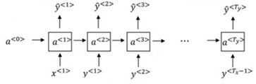
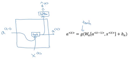
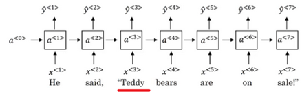
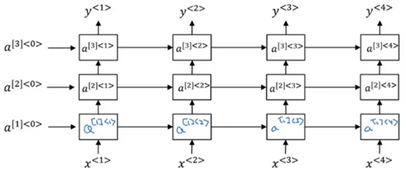
Lets build a RNN that solves name entity recognition task:
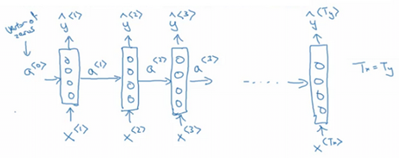
In this problem , In other problems where they aren't equal, the RNN architecture may be different .
is usually initialized with zeros, but some others may initialize it randomly in some cases.
There are three weight matrices here: with shapes:
:(NoOfHiddenNeurons,)
:(NoOfHiddenNeurons,NoOfHiddenNeurons)
:()
The weight matrix is the memory the RNN is tring to maintain from the previous layers.
A lot of papers and books write the same architecture this way:
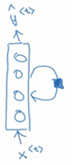
Its harder to interpreter. Its easier to roll this drawing to the unrollled version we have
descried.
In the discussed RNN architecture, the current output depends on the previous inputs and activations.
Lets have this example, He said,"Teddy Roosevelt was a great president". In this example Teddy is a person name but we know that from the word President that came after Teddy not from He and said that is befoere it.
So limitation of the discussed architecture is that it learns from behind. To address this problem we will later discuss Bidirectional RNNs(BRNNs).
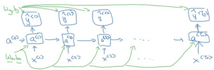
Now lets discuss the forward propagation equations on the discussed architecture.
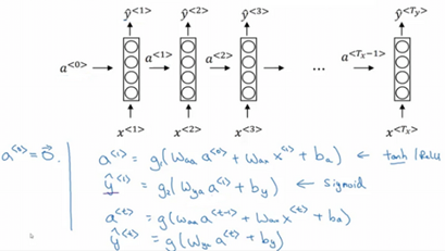
The activation function of a is usually tanh or RELU and for y depends on your task choosing some activation functions like sigmoid and softmax. In name entity recognition task we are solving, we will use Sigmoid because we only have two classes.
In order to help us develop complex RNN architectures, the last equations needs to be simplified a bit.
Simplified RNN notation:
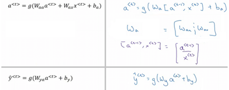
shape: (NoOf HiddenNeurons,NoOfHiddenNeurons+)
[a,] shape:(NoOfHiddenNeurons+,1)
Backpropagation through time
Lets see how backpropagation works with the RNN architecture we have developed.
Often, Deep Learning frameworks do backpropagation automatically for you. But its useful to know it works especially in RNNs.
Here is the graph:
Where are shared across each element in a sequence.
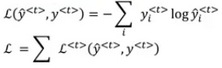
We will use the cross entropy loss function:
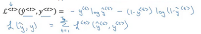
Where the first wquation is the loss for one element, and the loss for the whole sequence is given by the summation over all the calculated values.
Graph with losses:
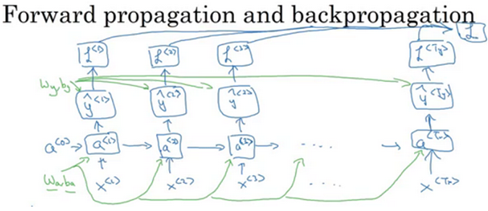
The backpropagation here is called backpropagation through time because of the passed activation a from one sequence element to another.
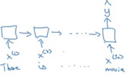
Different types of RNNs
So far we have seen only one RNN architecture in which equals always. In some other problems, they may not equal so we need different architectures.
The ideas inn this section was insprired by Andrej Karpathy blog. Mainly this image has all types:

The architecture we have descried before is called Many to Many.
In sentiment analysis problem, X is a text while Y is an integer that rangers from 1 to 5. The RNN architecture for that is Many to One as in Andrej Karpathy image.
A One to Many architecture application would be music generation.

Note that starting the second layer we are feeding the generated output back to the network.
There are another interesting architecture in Many To Many. Applications like machine translation inputs and outputs sequences have different lengths in most of the cases. So an alternative Many to Many architecture that fits the translation would be as follows:

Ther are an encoder and a decoder in the architecture. The encoder encodes the input sequence into one matrix and feed it to the decoder to generate the outputs. Encoder and decoder have different weight matrices.
There are another architecture which is the attention architecture which we will talk about in chapter 3.
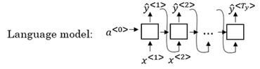
Language model and sequence generation
RNN do very well in language model problems. In this section we will build a language model using RNNs.
What is a language model
Lets say we are solving a speech recognition problem and some one says a sentence that
can be interpreted into to two sentences:
The apple and pair salad
The apple and pear salad
Pair and Pear sounds exactly the same, so how would a speech recognition application
choose from the two.
That's were the language model comes. It gives a probability for the two sentences and the application decides the best based on this probability.
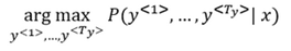
The job of a language model is given any sentence give a probability of that sentence. Also what is the next sentence probability given a sentence.
How to build language modeling with RNNs?
The first thing it to get a training set: Large corpus of target language text.
Then tokenize this training set by gettting the vocabulary and then ont-hot each word.
put an end of sentence token <EOS> with the vocabulary and include it with each
converted sentence. Also like we have mentioned before use the token <UNK> for the
unknown words.
Given the sentence "Cats average 15 hours of sleep a day.<EOS>"
In training time we will use this:
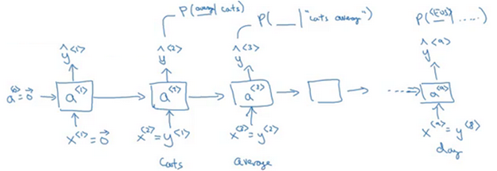
We pass to 0 vector – One hot – to the first layer.
The loss function is defined by cross entropy loss:
i is for all elements in the training set.
To use this model:
(1)For predicting the chance of next word, we feed the sentence to the RNN and then get the final ' hot vector and sort it by maximum probability
(2)For taking the probability of a sentence, we compute this:

This is simply feeding the sentence to the RNN and multiply the probability for the given
word in all the output hot encoded.
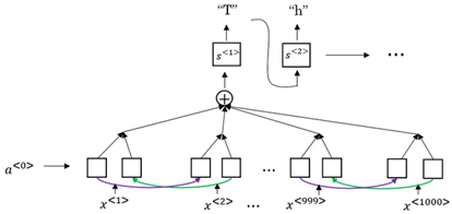
Sampling novel sequences
After a sequence model is trained on a language model, to check what the model has learned you can apply it on a sample novel sequence.
Let see the steps of how we can sample a novel sequence from a trained sequence language model:
-
Given this model:
-
we first pass =zeros vector, and =zeros vector.
-
Then we choose a prediction from using random distribution. For example it could be "The".
In Numpy this can be made using: numpy.random.choice
This is the line where you get a random sentences each time you run a novel sequence.
-
we pass the last predicted word with the calculated
-
we keep doing 3&4 steps for a fiexd length or until we get the<EOS> token.
-
You can reject any <UNK> token if you mind finding it in you output.
So far we have build a word level language model. A character level language model also can be made.
In the character level language model the vocabulary will contain [a-zA-Z0-9], space, and some special characters.
Cons of charater level language model compared to the word level language model:
There will be no <UNK> token
It can deal with any word
But mian disadvantage you will have a large sequence! and also more computationally expensive and harder to train.
Vanishing gradients with RNNs
One of the problem with naïve RNNs that it runs into vanishing gradient problems.
An RNN that proess a sequence data with the size of 10,000 time sets, has 10,000 deep layer! which is so hard to optimize.
To address the problem lets take an example. Suppose we are working with language modeling problem and there are two sequences that it tries to learn:
"The cat, which already ate………, was full"
"The cats, which already ate………,were full"
The dots represents many words
What we need to learn here that "was" came with "cat"and that "were" came with "cats". The naïve RNN will find it hard to get this relation.
As we have discussed in Deep neural networks, deeper networks are luckily to get into the vanishing gradient problem. In deep nets to compute the weights of the earlier layers you have to compute all the weights after these weights which causes the gradient to vanish. That also happens with RNNs with a long sequence size.
For computing the word "was", we need to compute the gradient for everything
behind,Multiply by fractions tends to vanish the gradient, while multiplication of large
number tends to explode it.
There for half of your weights may not be updated properly!
In the problem we descried it means that its hard for the network to memorize "was" word all over back to "cat". So in this case, the network won't be identify the singular/plural words so that it give it the right grammar word.
The conclusion is that RNNs aren't good in long term dependencies.
In theory, RNN are absolutely capable of handing such "long-term dependencies" A human could carefully pick parameters for them to solve toy problems of this form. Sadly in practice, RNNs don't seem to be able to learn them.
Vanishing gradients is tends to be the bigger problems with RNNs than the Exploding gradients problem. We will discuss how to solve it in the next sections..
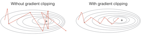
Exploding gradients can be easily seen when your weight values become NAN. So one of the ways solve exploding gradient is to apply gradient clipping means if your gradient is more than a threshold deal with gradient as a fixed value.
Extra:
Solution for the Exploding gradient problem:
Truncated back propagation.
Not to update all the weights in the way back.
Not optimal, You won't update all the weights.
Gradient clipping
Solution for the vanishing gradient problem:
Weight initialization
Like he initialization
Echo state networks
Use LSTM/GRU networks
Most popular
we will discuss it next.
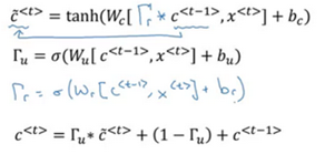
Gate Recurrent Unit(GRU)
GRU is an RNN type that can help solve the vanishing gradient problem and can remember the long term dependencies.
The basic RNN unit can be visualized to be like this:
We will represent the GRU with a similar drawings
Each layer in GRUs has a new variable c which is the memory cell. It can telll to wether memorize a something or not.
In GRUs,
Equations of the GRUs:
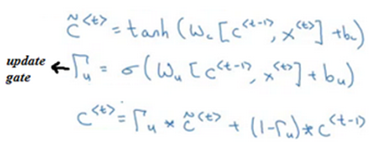
The update gate is between 0 and 1
To understand GRUs imagine that the update gate is either 0 or 1 most of the time
So we update the memory cell based on the update cell and the previous cell.
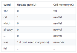
Lets take the cat sentence example and apply it to understand this equations:
Sentence:"The cat, which already ate………,was full"
We will suppose that U is 0 or 1 and is a bit that tells us if a singular word needs to be
memorized.
splitting the words and get values of C and U at each place:
Drawing for the GRUs

Drawings like this is so popular and makes it easier to understand GRUs and LSTMs. But
Andrew Ng finds its better to look at the equations.
Because the update gate U is usually a small number like 0.00001 GRUs doesn't suffer the vanishing gradient problem.
In the equation this makes in a lot of cases.
Shapes:
shape is (NoOfHiddenNeurons,1)
is the same as a
is the same as
is also the same dimensions of
The multiplication in the equations are element wise multiplication.
What has been descried so far is the Simplified GRU unit. Lets now describe the full one:
The full GRU contains a new gate that is used with to calculate the condidate C. The gate
tells you how relevance is
Equations:
Shapes are the same
So why we use these architectures, why don't we change them, how we know they will work, why not add another gate, why not use the simpler GRU instead of the full GRU; well researchers has experimented over years all the various types of these architectures with many many different versions and also addressing the vanishing gradient problem. They have found that full GRUs are one of the best RNN architectures to be used for many different problems. You can make you design but put in mind that GRUs and LSTMs are standards.
Long Short Term Memory(LSTM)
Other unit that can make you do long term dependences is an LSTM unit and its more powerfull and general than GRUs.
In LSTMs,
Here are the equations of an LSTM unit:
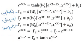
In GRUs we have an update gate u, a relevance gate r, and a condidate cell variables while in LSTMs we have an update gate U –Sometimes its called Input gate I -, a forget gate F, an output gate O and a candidate cell variables

Some Variants on LSTMs includes:
LSTM with peephole connections.
The normal LSTM with included with every gate.
There isn't a universal superir in choosing between LSTMs and its variants. Some win and some problems and some don't. One of the advantages of GRUs is that its simpler and can be used to build much bigger network but the LSTM is more powerful and general as we said.
Bidirectional RNN
There are still some ideas to make a powerfull sequence model. One of them is bidirectional RNNs and another is Deep RNNs.
As we saw before, here are an example on Name entity recognition:
The name Teddy cannot be learned from He and said, but can be learned from bears.
BRNNs fixes this issue.
Here are BRNNs architecture:
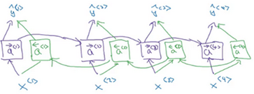
Hint that BRNNs are acyclic graph!
The forward propagation goes from left to right, and from right to left. It learns from both sides.
To make predictions we use y^<t> by using the two activations that comes from left and right.
The blocks here can be any RNN block including the basic RNNs,LSTMs,or GRUs
For a lot of NLP or text processing problems, a BRNN with LSTM appears to be commonly used.
The disadvantage of BRNNs that you need the entire sequence before you can process it.For example in live speech recognition if you used BRNNs you will need to wait for the person who speaks to stop to take the entire sequence and then make your predictions.
Deep RNNs
In a lot of cases the standard one layer RNNs will solve your problem. But in some problems its useful to stack some RNN layers to make a deeper network.
For example,a deep RNN with 3 layers would look like this:
In feed forward deep nets we can have till 100 ro 200 layer and this would be a so big network. In deep RNNs stacking 3 layers is considered deep and already expensive.
In some cases you might see a deep network that are connected after recurrent cell.
Back propagation with RNNs
In modern deep learning frameworks, you only have to implement the forward pass, and the framework takes care of the backward pass, so most deep learning engineers do not need to bother with the details of the backward pass.
Natural Language Processing & Word Embeddings
Natural language processing with deep learning is an important combination. Using word vector representations and embedding layers you can tarin recurrent neural networks with outstanding performances in a wide variety of industries. Example of applications are sentiment analysis, named entity recognition and machine translation.
Introduciton to Word Embeddings
word representation
NLP has been revolutionized by deep learning and especially be RNNs and deep RNNs.
Word embedding is a way of representing words. It lets your algorithm automatically understand the analogies between words like "king" and "queen".
So far we have defined our language by a vocabulary. Then represented our words with one hot vector that represent the word in the vocabulary.
An image example would be:
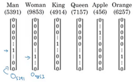
We will use the annotation for any word that is represented with one hot like in the
image.
One of the weaknesses of this representation is that it treats a words as a thing that itself
and it doesn't allow an algorithm to generalize across words.
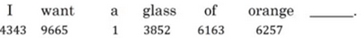
For example:" I want a glass of orange___", a model should predict the next word as
Juice
A similar example "I want a glass of apple____", a model won't easily predict juice
here if it doesn't trained on it. And if so the two examples aren't related although
orange and apple are similar.
Inner product between any hot encoding word is zero. Also the distance between them
are the same.
So, won't it be nice if instead of a one-hot presentation we can instead lean a featurizd representation with each of these words: Man, Woman, King, Queen, Apple, and orange?

Each word will have a 300 feature float point number for example.
Each word column will be 300 dimensional vector which will be representation.
We will use the notation to describe Man word features vector.
Now if we went to the example we descried again:
"I want a glass of orange____"
"I want a glass of apple______"
Orange and apple now shares a lot of similar features which makes it easier for an
algorithm to generalize between them.
We call this representation Word embeddings.
To visualize word embeddings we use t-SNE algorithm to reduce the features to 2 dimensions which make it easy to visualize
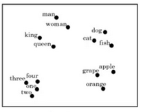
You will get a sense that more related words distance are smaller than other distances.
The word embeddings came from that we need to embed a unique vector inside an n dimensions.
Using word embeddings
Lets see how we can take the feature representation we have extracted from each word and apply it in Name entity recognition problem.
Given this example – From name entity recognition:
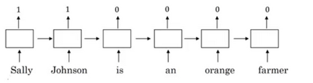
Sally Johnson is a persons name.
After training on this sentence the model should find out that the sentence "Robert Lin is an apple farmer" contains Robert Lin as a name, as apple and orange has near representations.
Now if you have tested your model with this sentence "Mahmound Badry is a durian cultivator" the network should learn the name even if it hasn't seen the word durian before. That's the power of word representations.
The algorithms that are used to learn word embeddings can exterminate billions of unlabeled text- for example 100 billion- words and learn the representation from them.
Transfer learning and word embeddings:
-
Learn word embeddings from large text corpus. say 100 billion word
Or download pre-trained embedding online
-
Transfer embeddings to new task with smaller training set. say 100k word.
-
Optimal: Continue to finetune the word embeddings with new data.
-
This can be done if your samller training set are big enough.
-
Also one of the advantages of using word embeddings is that it reduces the size of the input!
10,000 one hot compared to 300 features vector.
Word embeddings has an interesting relationship to the face recognition task:

In this problem we encode each face into a vector and then check how similar is these
vectors.
The word encode and embeddings has a similar meaning here.
In the word embeddings task, we are getting a vector say from to for each word
in our vocabulary. We will discuss the algorithm in the next sections.
Properties of word embeddings
One of the most fascinating properties of word embeddings is that they can also help with analogy reasoning. Analogy reasoning is one of the most important applications of NLP.
Analogies example:
Given this word embeddings table:
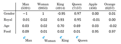
Can we conclude this relation:
ManèWoman
Kingè??
Lets subtract from . This will equal the vector [-2 0 0 0]
Similar -=[-2 0 0 0]
So the difference is about the gender in both.
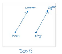
This vector represents the gender.
This drawing is 2D visualization of the 4D vector that has benn extracted by t-SNE
algorithm. It was drawing for just clarification!Don't rely on t-SNE algorithm in
finding parallels.
So we can reformulate the problem to finding:
-
It can also represented mathematically by:

It turns out that is the best solution here that get the similar vector.
Cosine similarity:
Equation:
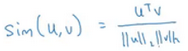
The top part represents the inner product of u and v vectors. That will be large if the vectors are so similar.
We can use this equation to calculate the similarities between word embeddings and on
the analogy problem where u= and v=
Embedding matrix
When you implement an algorithm to learn a word embedding, what you end up learning is an embedding matrix.
Lets take an example:
Suppose we are using 10,000 words as our vocabulary.
The algorithm should extract a matrix E of the shape(300,10,000) in case we are extracting
300 features.(300,10,001) if we have <UNK> token.

If is the one hot encoding of the word orange, then E* equals which
shape is(300,1)
Generally E*=
In the next sections you will see that we first initialize E randomly and then try to learn all the parameters of this matrix.
In practice its not efficient to use a dot multiplication when you are tyring to extract the embedding of a specific word, instead we will use slicing to slice a specific column. In keras there are a embedding layer that extracts this column with no multiplications!
Learning Word Embedding: Word2vec & Glove
Learning word embeddings
Lets start learning some algorithm that learns the word embeddings
At start, word embeddings algorithm – with deep learning – were complex but then it started simpler and simpler.
We will start by learning the complex examples to make more sense.
Neural Language model:
Lets start by example:
We want to build a language model so that we can predict the next word.
So we use this neural network to learn the language model
We get by E*
NN layer has parameters w1 and b1 while softmax layer has parameters w2 and b2
Input dimension is (300*6,1) if we the window size is 6.
Here we are optimizing E matrix and layers parameters.
This model was build on 2003 and tends to work very well to get the embeddings.
In the last example we took a window of 6 words that fall behind the word that we want to predict. There are other choices when we are trying to learn word embeddings
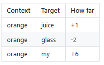
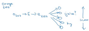
Suppose we have the example:"I want a glass of orange juice to go along with my cereal"
To learn juice, Choice of Context are:
Last 4 words
We use a window of last 4 words- 4 is the best -,"a glass of orange" and try to
predict the next word from it.
4 words on the left and on the right.
"a glass of orange" and "to go along with"
Last 1 word
"orange"
Nearby 1 word.
"glass" word is near juice
The idea of skip grams models
The idea is so simpler and works remarkably well
We will talk about this in the next section.
Word2Vec
Before presenting Word2Vec, lets talk about Skip-grams:
For example if we have the sentence:"I want a glass of orange juice to go along with
my cereal"
We will choose Context and target.
The target is choose randomly based on a window with a specific size.
We have converted the problem into a supervised problem.
This is not an easy learning problem because within -10/+10 words for example is hard.
We want to learn this to get our word embeddings model.
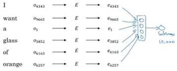
Word2Vec model:
Vocabulary size=10,000 word
Lets say that the context word are c and the target word are t
We want to learn c to t
we get by E.
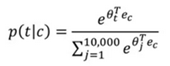
we then use a soft layer to get p(t|c) which is y^
Also we will use the cross-entropy loss function
This model is called skip-grams model.
The last model has a problem with the softmax classifier:
Here we are summing 10,000 numbers which corresponds to the number of words in
our vocabulary.
If this number is larger say 1million, the computation will beecome so slow.
The solution for the past problem is to use "Hierachical softmax classifier" which works as a tree classifier.
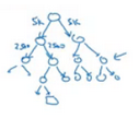
In practice the hierarchical softmax classifier doesn't use a balanced tree like the drawn one. Common words are in the top and less common are in the buttom.
How to sample the context c?
One way is to choose the context by random from your corpus
If you have done it that way, there will be frequent words like "the, of, a , and, to,.." that
can dominate other words like "orange, apple,Mahmoud,…"
So in practice, we don't take the context uniformly random, instead there are some
heuristics(启发式) to balance the common words and the none common words.
Negative Sampling
Negative sampling allows you to do something similar to the Skip-Gram model, but with a much more efficient learning algorithm. We will create a different learning problem.
Given this example:
"I want a glass of orange juice to go along with my cereal"
The sampling will look like this:

we get positivi example by using the same skip-grams technique, a fixed window that
goes around.
To generate a negative example, we pick a word randomly from the vocabulary.
Notice that we got "of" although it was appeared in the same sentence
So the steps to generate the samples are:
-
pick a positive context
-
pick a negative context from the dictionary
K is recommended to be from 5 to 20 in small datasets. For larger ones 2 to 5.
We will have a k negative examples to 1 positive ones in the data we are collecting.
Now lets define the model that will learn this supervised learning prolem:
Lets say that the context word are c and the word are t and y is the target.
We will apply the simple logistic regression model.
The logistic regression model can be drawn like this:
So we are like having 10,000 binary classification problem, and we only train k+1 classifier
of them in each iteration
Now how to select negative samples:
We can sample according to empirical frequencies in words corpus which means
according to how often different words appears. But the problem with that is that we will
have more frequent words like the,of,and…
The best is to samplewith this equation—According to authors--:
GloVe word vectors
GloVe is another algorithm for learning the word embeddings, its thesimplest of them.
This is not used much as word2vec or gram models, but is has some enthusiasts because of its simplicity.
GloVe stands for Global vectors for word presentation.
Given this example:
"I want a glass of orange juice to go along with my cereal"
We will choose a context and a target from the choices we have mentioned in the previous sections.
Then we will calculate this for every pair, =# times t appears in context of c
if we choose a window pairs, but they will not equal if we choose the previous words fo rexample. In GloVe they use a window which means they are equal
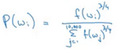
The model is defined like this:
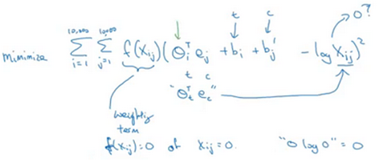
f(x) is given to help with the log 0 problem, Also it gives a weights for some words. For stop words like this,is,the it gives it a low weight, also for words that doesn't occur so much.
ceta and e are symmetric which helps getting the final word embedding
Conclusion on word embeddings:
If this is your first try, you should try to download a pretrained model that has been made
and actually works best.
If you have enough data, you can try to implement one of the avaliable algorithm
Because word embeddings are very computationally expensive to train, most ML
practitions will load a pretrained set of embeddings.
A final note that you can't guarantee that the axis used to represent the features will be
weill-aligned with what might be easily humanly axis like gender,and royal and age.
Application using Word Embeddings
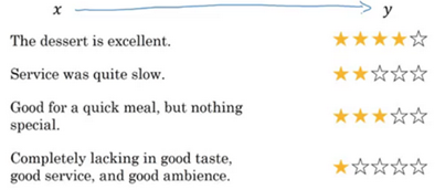
Sentiment Classification
As we have discussed before, Sentiment classification is the process of finding if a text has a positive or a negative review. Its so useful in NLP and is used in so many application. An example would be:
One of the challenges with it, is that you might haven't a huge labeled training data for it, but using word embeddings can help getting rid of this.
The common dataset size varies from 10,000 to 100,000 words.
A simple sentiment classification model would be like this:
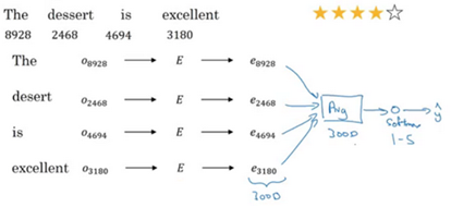
The embedding matrix may have been trained on say 100 billion words.
Number of features given a word is 300
We can use sum or average given all the words then pass it to a softmax classifier. That
makes this classifier works for short or long sentences.
One of the problems with this simple model is that it ignores words order! for example "Completely lacking in good taste, good service, and good ambience" has the word good 3 times but it's a negative review!
A better model uses an RNN for solving this problem:
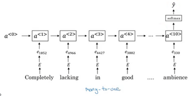
And so if you train this algorithm, you end up with a pretty decent sentiment classification
algorithm.
Also it will generalize even if words aren't in your dataset, for example the sentencte
"Completely absent of good taste, good service , and good ambience" will be the same
as the trained word!
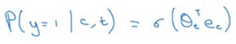
Debiasing word embeddings
We want to make sure that our word embeddings free from undesirable forms of bias, such as gender bias, ethnicity bias and so on.
A horrifying result on a trained word embeddings in the context of Analogies:
Man: Computer_programmer as Woman:Homenaker
Father: Doctor as Mother:Nurse
Word embeddings can reflect gender, ethnicity, age, sexual orientation, and other biases of text used to train the model.
Learning algorithm by general is making an important decisions! and it mustn't be biased
Andrew think we actually have better ideas for quickly reducing the bias in AI than for quickly reducing the bias in the human race, although it still needs a lot of work to be donw.
Addressing bias in word embeddings steps:
Given this learned embeddings:
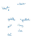
we need to solve the gender bias here. The steps we will discuss can help solve any bias
problem but we are focusing here on gender bias.
Here are the steps:
-
Identify the direction:
Calculate the difference between

Choose some k difference and average them.
This will help you find this:
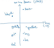
By that we have found the bias direction which is 1D vector and the non-bias vector which is 299D
-
Neutralize: For every word that is not definitional, project to get rid of bias.
Babysitter and doctor needs to be neutral so we project them on nonbias with the direction of the bias:
After that they will be equal in the term of gender.
To do this the authors of the paper trained a classifier to tell the words that
needs to be neutralized or not.
-
Equalize pairs
We want each pair to have difference only in gender. Like:
Grandfather - Grandmother
He – She
Boy – Girl
We want to do this because the distance between grandfather and babysitter is bigger than babysitter and grandmother:

To do that, we move grandfather and grandmother to a point where they will be in the middle of the non-bias axis.
There are some words you need to do this for in your steps. The size of these words are relatively small.
Sequence models & Attention mechanism
Sequence models can be augmented using an attention mechanism. This algorithm will help your model understand where it should focus its attention given a sequence of inputs. This week, you will learn about speech recognition and how to deal with audio data.
Various sequence to sequence architectures
Basic Models
In this section we will learn about sequence to sequence –Many to Many – models that are useful in various applications includes machine translation and speech recognition
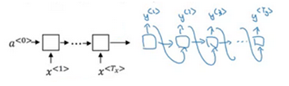
Lets start by the basic model:
Given this machine translation problem in which X is a French sequence and Y is an
English sequence.
Our architecture will include encoder and decoder.
The encoder is built with RNNs – LSTM or GRU are included – and takes the input
sequence and then outputs a vector that should represent the whole input.
After that the decoder network, are also built with RNNs and outputs the ouput sequence
using the vector that has been built by the encoder.
With an architecture similar to the one previously mentioned works for image captioning problem:
In this problem X is an image, while Y is a sentence.
The model architecture image:

The architecture uses a CNN pretrained AlexNet as an encoder for the image, and the
decoder is an RNN.
Picking the most likely sentence
There are some similarities betweenthe language model we have learned previously, and the machine translation model we have just discussed, but there are some difference as well.
The language model we have learned as so similar to the decoder of the machined translation model, except for

The problems formations also are different:
In language model: P(y<1>, ....y<Ty>)
In machine translation: P(y<1>, ....y<Ty> | y<x>, ....x<Tx>)
What we don't want in machine translation model,is not to sample the output at random. This may provide some choice as an output. Sometimes you may sample a bad output.
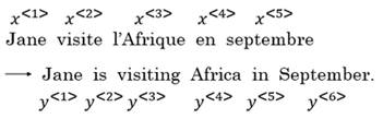
Example:
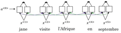
X="Jane visite I'Afrique en septembre"
Y may be:
Jane is visiting Africa in September.
Jane is going to be visiting Africa in September.
In september, Jane will visit Africa.
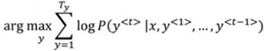
So we need to get the best ouput, this can be take by the equation:
The most common algorithm is the beam search, which we will explain in the next section.
Why not use greedy search? why not get the best choices each time?
It turns out that this approach doesn't really work!
Lets explain it with an example:
The best output for the example we talked about is "Jane is visiting Africa in
September."
Suppose that you when you are choosing with greedy approach, the first two words
were "Jane is", the word that may come after that will be "going" as "going" is the
most common word that comes after "Noun is" so the result may look like this:"Jane
is going to be visiting Africa in September." and that isn't the best/optimal solution.
So what is bettern than greedy approach, is trying to gt an approximate solution, that will try to maximize the output.
Beam Search
Beam search is the most widely used algorithm to get the best output sequence. It's a heuristic search algorithm.
To illustrate the algorithm we will be stick with the example from the previous section. We need Y="Jane is visiting Africa in September."
The algorithm has a parameter B which is the beam width. Lets take B=3 which means the algorithm will get 3 outputs at a time.
For the first step you will get["in","jane","september"] words that are the best condidates.
Then for each word in the fist output,, get B words from the 3 where the best are the result of multiplying both probabilities. So we will have the["In September","jane is","jane visit"]. Notice that we automatically ignored September.
Repeat the same process and get the best B words for ["September","is","visit"] and so on.
In this algorithm, keep only B instances of your network
If B=1 this will become the greedy search.
Refinements to Bean Search
In the previous section we have discussed the basic beam search. In this section we will try to do some refinements to it to work even better.
The fist thing is Length optimization
In beam search we are trying to optimize:
And to do that we multiply:
P(y<1> | x) * P(y<2> | x, y<1>) * ..... P(y<t> | x, y<y(t-1)>)
Each probability is a fraction. Also maybe a small fraction.
Multiplying small fractions will cause a numerical overflow! Meaning that it's too small
for the floating part representation in your computer to store accurately.
So in practice we use summing logs instead of multiplying directly.
But theres another problem. The two optimization functions we have mentions tends to
find small sequences! Because multiplying a lot of fractions gives a smaller value.
So theres another change, by dividing by the number of elements in the sequence.
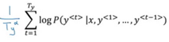
alpha is a hyper parameter to tune.
If alpha=0, Then its like we do nothing.
If alpha=1, Then its like we are using full sequence length.
In practice alpha=0.7 is a good thing.
The second thing is who can we choose best B?
The larger B, the larger possibility, the better are the results. But it will be more
computationally expensive.
In practice, you might see a in the production sentence B=10.
B=100,B=1000 are uncommon.
Unlike exact search algorithm like BFS(Breadth First Search) of DFS(Depth Fist Search).
Beam Search runs fater but is not guaranteed to find exact solution.
Error analysis in beam search
We have talked before on Error analysis in Structuring Machine Learning Projects Projects chapter. We will apply these concepts to improve our beam search algorithm
We will use error analysis to figure out if the B hyperparameter of the beam search is the problem – because it doesn't get an optimal solution – or to in other hyperparameters like the RNN parameters.
Lets take an example:
Our examples information:
X="Jane visite I'Afrique en septembre."
Y*="Jane visits Africa in September."
Y^="Jane visited Africa last September"
Our model that has produced a sentence that are different in meaning because of the
word "last"
We now want to know who to blame, the RNN or the beam search.
To do that, we calculate P(y* | X) and P(y^ | X). There are two cases:
Case 1 (P(y* | X) > P(y^ | X)):
Conclusion: Beam search is at fault.
Case 2 (P(y* | X) <= P(y^ | X)):
Conclusion: RNN model is at fault.
The error analysis process is as following:
You choose N error examples and make the following table:
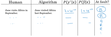
B for beam search, R is for the RNN.
Get counts and decide.
BLEU Score
One of the challenges of machine translation, is that given a sentence in a language there are one or more possible good translation in another language. So how do we evaluate our results?
The way we this is by using BLEU score. BLEU stands for bilingual evaluation understudy.
The intuition is so long as the machine generated translation is pretty close to any of the reference procide by humans, then it will get a high BLEU Score.
Lets take an example:
X="Le chat est sur le tapis."
Y1="The cat is on the mat."
Y2="There is a cat on the mat."
Suppose that the machine outputs:"the the the the the."
One way to evaluate the machine output is to look at each word in the output and check
it in the references. This is called precision:
precision=7/7 because the appeared in Y1 or Y2
This is not a useful measure!
We can use a modified precision in which we are looking for the reference with the
maximum number of a particular word and set the maximum appearingof this word to
this word to this number. So:
modified precision=2/7 because the max is 2 in Y1
We clipped the 7 times by the max which is 2.
The problem here is that we are looking at one word at a time, we may need to look at
pairs
Another example (BLEU score on bigrams)
The n-grams typically are collected from a text or speech corpus. When the items are
words, n-grams may also be called shingles. An n-gram of size 1 is referred to as
"unigram"; size 2 is a "bigram"(or, less commonly,a "digram"); size 3 is a "trigram".
X="Le chat est sur le tapis"
Y1="The cat is on the mat."
Y2="There is a cat on the mat"
Suppose that the machine outputs:"The cat the cat on the mat."
The bigrams in the machine output:
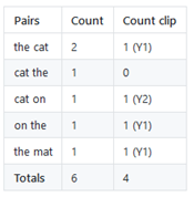
Score=Count clip/Count=4/6
So here are the equations for the n-grams:
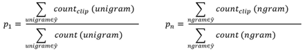
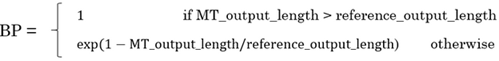
Lets put this together to formalize the BLEU score:
Bleu score on n-grams only
Combined Bleu score equation:

For example if we want Bleu for 4, we compute, we compute P1, P2, P3, P4 and then average
them and take the exp.
Another equation is BP penalty which stands for brevity penalty. It turns out that if a
machine outputs a small number of words it will get a better score so we need to handle
that.
Blue Score is has several open source implementations and used in variety of systems like machine translation and image captioning.
Attension Model Intuition
So far we are using sequence to sequence models with an encoder and decoders. There are a technique called attention which make these models even better.
The attention algorithm, the attension idea has been one of the most influential ideas in deep learning.
The problem of long sequence:
Given this model, inputs, and outputs:
The encoder should memorize this long sequence into one vector, and the decoder has
to process this vector to generate the translation.
If a human would translates this sentence, he wouldn't read the whole sentence and
memorize it then try to translate it. He translates a part at a time.
The performance of this model decreases if a sentence is so long.
We will discuss the attension model that works like a human that looks at parts at a time.
That will significantly increase the accuracy even with bigger sequence:
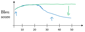
Blue is the normal model, while green is the model with attention mechanism.
In this section we will give just some intuitions about the attention model and in the next section we will discuss its details.
At first the attention model was developed for machine translation but then other application used it like computer vision and new architectures like Neural Turing machine.
Now for the intuition:
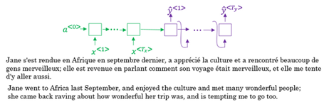
Suppose that our decoder is a bidirectional RNN:
We gave the French sentence to the encoder and it should generate a vector that
represents the inputs.
Now to generate the first word in English which is "Jane" we will make another RNN
which is the decoder.
attention weights are used to specify which words are needed when to generate a word.
So to generate "jane" we will look at "jane","visite","I'Afrique"
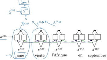
alpha1,1, alpha1,2, and alpha1,3 are the attention weights used.
And so to generate any word there will be a set of attention weights that controls words
we are looking at right now.
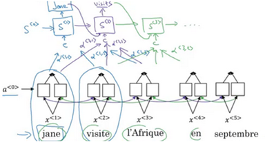
Attention Model
Lets formalize the intuition from the last section into the exact details on how this can be implemented.
First we will have an bidirectional RNN – most common is LSTMs – that encodes French language:

For learning purpose, lets assume that a<t> will include the both directions.
We will have an RNN to extract the output using a context c which c is computer using the attention weights. This denotes how much information do it needs to look in a<t>
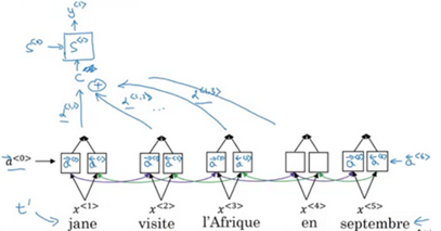
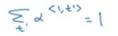
Sum of the attentionweights for each element in the sequence should be 1:
Also the context c are calculated using this equation:
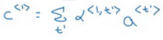
Lets see how can we compute the attention weights:
So alpha<t, t'> = amount of attention y<t> should pay to a<t'>
Like for example we payed attention to the first three words through alpha<1,1>,
alpha<1,2>, alpha<1,3>
We are going to softmax that attention weights so that their sum is 1:
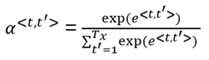
Now we need to know how to calculate e<t, t'>.We will compute e using a small neural
network:

s<t-1> is the hidden state of the RNN s, and a<t'> is the activation of the other bidirectional
RNN.
One of the disadvantages of this algorithm is that it takes quadratic time or quadratic cost to run.
One fun way to see how attention works is by visualizing the attention weights:
Speech recognition – Audio data
Speech recognition
The rise of accurate speech recognition was the most exciting work done in sequence to sequence deep learning models.
Lets define the speech recognition problem:
X: audio clip
Y: transcript
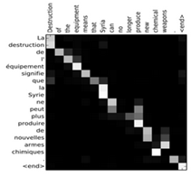
If you plot an audio clip it should look like this:
The horizontal axis is time while the vertical is changes in air pressure.
What really is an audio recording? A microphone records little variations inn air pressure
over time, and it is these little variations in air pressure that your ear also perceives as
sound. You can think of an audio recording is a long list of numbers measuring the little
air pressure changes detected by the microphone. We will use audio sampled at 44100Hz.
This means the microphone gives us 44100 numbers per second. Thus, a 10 second audio
clip is represented by 441000 numbers
It is quite difficult to work with "raw" representation of audio.
Because even human ear doesn't process raw wave forms, the human ear can process
different frequencies.
There's a common preprocessing step for an audio to generate a spectrogram which
works similarly to human ears.
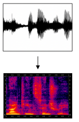
The horizontal axis is time while the vertical is frequencies. Intensity of different
colors shows the amount of energy.
A spectrogram is computed by sliding a window over the raw audio signal, and calculates
the most active frequencies in each window using a Fourier transform.
In the past days, speech recognition systems was built withphonemes that are a hand
engineered basic units of sound. Linguists use to gypothesize any writing down audio in
terms of phonemes which they though would be the best way to do speech recognition.
End to end deep learning found that phonemes was no longer needed. One of the things
that made this possible is the large audio datasets.
Research papers has 300-3000 hours while the best commercial systems are now trained
on over 100,000 hours of audio
You can build an accurate speech recogniition system using the attention model that we have descried in the previous section:
One of the methods that seem to work well is CTC cost which stands for "Connectionist temporal classification:
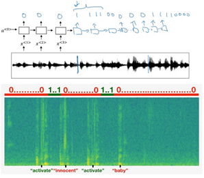
Trigger word Detection
With the rise of deep learning speech recognition, there are a lot of devices that can be waked up by saying some words with your voice. These systems are called trigger word systems.
For example, Alexa –a smart device made by amazon – can answer your call "Alexa What time is it" and then Alexa will reply you
Trigger word detection system includes:

Now the trigger word detection literature is still evolving so there actually isn't a single universally agreed on algorithm for trigger word detection yet. But lets discuss an algorithm that can be used.
Let now build a model that can solve this problem:
X: audio clip
X will be labels 0 or 1.0 represents the non trigger word, while 1 is that trigger word that
we need to detect.
The model architecture can be like this:
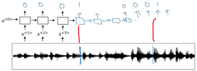
The vertical lines in the audio clip represents the trigger words. The corresponding
to this will be 1.
One disadvantage of this is the imbalanced dataset outputs. There will be a lot of zeros
and little ones.
A hack to solve this is to make an output a few ones for several times or for a fixed period
of time before reverting back to zero.
Extras
Machine Translation Attention Model(From notebooks)
The model is built with keras layers
The attention model

