版权声明:本文为博主原创文章,转载时请注明作者和出处。 https://blog.csdn.net/A_a_ron/article/details/79004163
前言
Keras源码中附有一个examples的文件夹,里面包含一些使用Keras进行编写的常用的神经网络模型,如CNN、LSTM、ResNet等。这些例子基本上是Keras学习入门必看的,作为Keras的学习者,就在这里记录一下examples中的代码解析,一为自身记忆,二为帮助他人。
源码
这里解析的源码是变分自动编码器(variational autoencoder,VAE),其是标准自动编码器的一个升级版本。与标准自动编码器相比,VAE在编码器阶段添加了一个约束,使产生的code服从单位高斯分布。关于VAE的介绍可参考这里。
VAE的示意图如下:
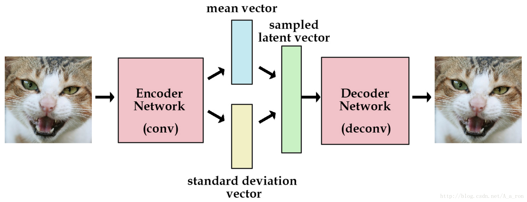
VAE的示例代码在Keras中的路径为Keras/examples/variational_autoencoder.py。整个网络是由多层感知机构成的,非卷积层。上面示例图中写的是卷积,两者基本结构一致。
examples中的variational_autoencoder_deconv.py文件中的代码是VAE的卷积网络实现的形式,两者运行的结果很类似,代码上也很接近,大家可以参照这个来理解卷积网络版本的VAE。
#导入相关包
import numpy as np
import matplotlib.pyplot as plt
from scipy.stats import norm

from keras.layers import Input, Dense, Lambda, Layer
from keras.models import Model
from keras import backend as K
from keras import metrics
from keras.datasets import mnist
#整个网络的维度变化为:784->256->2->256->784
batch_size = 100
#原始输入维度,28*28=784
original_dim = 784
#编码后的code的维度
latent_dim = 2
#中间隐藏层的维度
intermediate_dim = 256
#迭代50次
epochs = 50
#初始化时的标准差
epsilon_std = 1.0#编码器的结构
x = Input(shape=(original_dim,))
h = Dense(intermediate_dim, activation='relu')(x)
# mean vector
z_mean = Dense(latent_dim)(h)
# standard deviation vector
z_log_var = Dense(latent_dim)(h)#使用均值变量(mean vector)和标准差变量(standard deviation vector)合成隐变量
def sampling(args):
z_mean, z_log_var = args
#使用标准正态分布初始化
epsilon = K.random_normal(shape=(K.shape(z_mean)[0], latent_dim), mean=0.,stddev=epsilon_std)
#合成公式
return z_mean + K.exp(z_log_var / 2) * epsilon
# note that "output_shape" isn't necessary with the TensorFlow backend
#z即为所要求得的隐含变量
z = Lambda(sampling, output_shape=(latent_dim,))([z_mean, z_log_var])# we instantiate these layers separately so as to reuse them later
# 解码器的结构
decoder_h = Dense(intermediate_dim, activation='relu')
decoder_mean = Dense(original_dim, activation='sigmoid')
h_decoded = decoder_h(z)
#x_decoded_mean 即为解码器输出的结果
x_decoded_mean = decoder_mean(h_decoded)# Custom loss layer
#自定义损失层,损失包含两个部分:图片的重构误差(均方差Square Loss)以及隐变量与单位高斯分割之间的差异(KL-散度KL-Divergence Loss)。
class CustomVariationalLayer(Layer):
def __init__(self, **kwargs):
self.is_placeholder = True
super(CustomVariationalLayer, self).__init__(**kwargs)
def vae_loss(self, x, x_decoded_mean):
xent_loss = original_dim * metrics.binary_crossentropy(x, x_decoded_mean)#Square Loss
kl_loss = - 0.5 * K.sum(1 + z_log_var - K.square(z_mean) - K.exp(z_log_var), axis=-1)#KL-Divergence Loss
return K.mean(xent_loss + kl_loss)
def call(self, inputs):
x = inputs[0]
x_decoded_mean = inputs[1]
loss = self.vae_loss(x, x_decoded_mean)
self.add_loss(loss, inputs=inputs)
# We won't actually use the output.
return x有关损失函数的推导,感兴趣的可看这篇论文的推导
#将损失层加入网络
y = CustomVariationalLayer()([x, x_decoded_mean])
vae = Model(x, y)
vae.compile(optimizer='rmsprop', loss=None)
# train the VAE on MNIST digits
#使用MNIST数据集进行训练
(x_train, y_train), (x_test, y_test) = mnist.load_data()
#图像数据归一化
x_train = x_train.astype('float32') / 255.
x_test = x_test.astype('float32') / 255.
#将图像数据转换为784维的向量
x_train = x_train.reshape((len(x_train), np.prod(x_train.shape[1:])))
x_test = x_test.reshape((len(x_test), np.prod(x_test.shape[1:])))#模型训练设置
vae.fit(x_train,
shuffle=True,
epochs=epochs,
batch_size=batch_size,
validation_data=(x_test, None))至此,整个网络的构建和训练都结束,下面为测试的代码。
# build a model to project inputs on the latent space
#编码器的网络结构,将输入图形映射为code,即隐含变量
encoder = Model(x, z_mean)
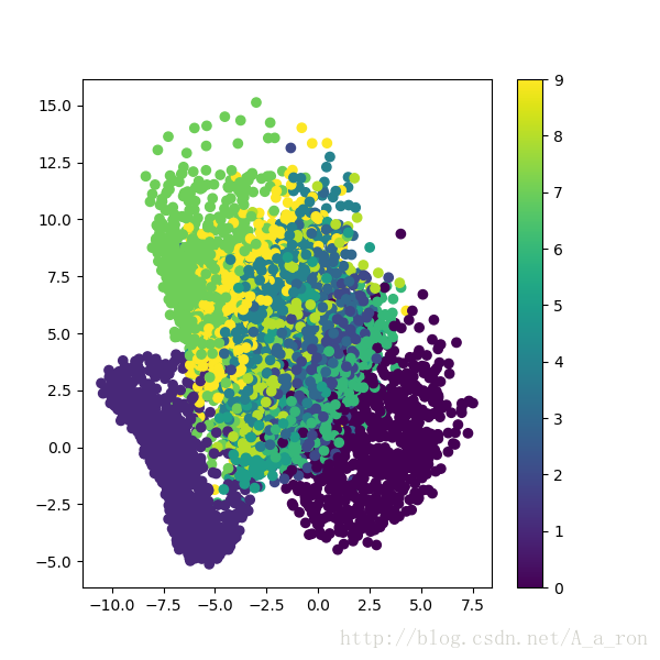
# display a 2D plot of the digit classes in the latent space
#将所有测试集中的图片通过encoder转换为隐含变量(二维变量),并将其在二维空间中进行绘图
x_test_encoded = encoder.predict(x_test, batch_size=batch_size)
plt.figure(figsize=(6, 6))
plt.scatter(x_test_encoded[:, 0], x_test_encoded[:, 1], c=y_test)
plt.colorbar()
plt.show()测试集图像经过encoder之后在二维空间中的分布如下:
# build a digit generator that can sample from the learned distribution
#构建一个解码器,用于将隐变量解码层图片
decoder_input = Input(shape=(latent_dim,))
_h_decoded = decoder_h(decoder_input)
_x_decoded_mean = decoder_mean(_h_decoded)
generator = Model(decoder_input, _x_decoded_mean)
# display a 2D manifold of the digits
#绘制一个15个图像*15个图像的图
n = 15 # figure with 15x15 digits
#每个图像的大小为28*28
digit_size = 28
#初始化为0
figure = np.zeros((digit_size * n, digit_size * n))
# linearly spaced coordinates on the unit square were transformed through the inverse CDF (ppf) of the Gaussian
# to produce values of the latent variables z, since the prior of the latent space is Gaussian
# 生成因变量空间(二维)中的数据,数据满足高斯分布。这些数据构成隐变量,用于图像的生成。
#ppf为累积分布函数(cdf)的反函数,累积分布函数是概率密度函数(pdf)的积分。np.linspace(0.05, 0.95, n)为累计分布函数的输出值(y值),现在我们需要其对应的x值,所以使用cdf的反函数,这些x值构成隐变量。
grid_x = norm.ppf(np.linspace(0.05, 0.95, n))
grid_y = norm.ppf(np.linspace(0.05, 0.95, n))有关scipy中的ppf函数可查看这里
#绘图
for i, yi in enumerate(grid_x):
    for j, xi in enumerate(grid_y):
        z_sample = np.array([[xi, yi]])#add by weihao: 1*2
        x_decoded = generator.predict(z_sample)
        digit = x_decoded[0].reshape(digit_size, digit_size)#add by weihao: the generated image
        figure[i * digit_size: (i + 1) * digit_size,
               j * digit_size: (j + 1) * digit_size] = digit

plt.figure(figsize=(10, 10))
plt.imshow(figure, cmap='Greys_r')
plt.show()
使用构建的隐含变量解码出的图像如下图所示:
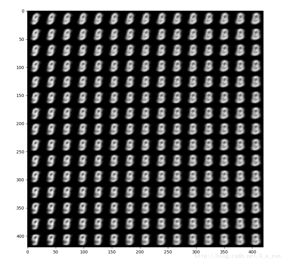
可以看出,还是有一定的误差的。
附VAE的原始论文:Auto-Encoding Variational Bayes