TensorFlow_线性回归实现

数据集和前面一篇一样。

#!/usr/bin/env python3
# -*- coding: utf-8 -*-

import numpy as np
import tensorflow as tf
import matplotlib.pyplot as plt

if __name__ == '__main__':
    # 给参数赋值
    learning_rate = 0.01
    training_epochs = 1000
    display_steps = 50

    train_X = np.array([3.3, 4.4, 5.5, 6.71, 6.93, 4.168, 9.779, 6.182, 7.59, 2.167, 7.042, 10.791, 5.313, 7.997, 5.654, 9.27, 3.1])
    train_Y = np.array([1.7, 2.76, 2.09, 3.19, 1.694, 1.573, 3.366, 2.596, 2.53, 1.221, 2.827, 3.465, 1.65, 2.904, 2.42, 2.94, 1.3])
    n_samples = train_X.shape[0]

    # 定义数据流图上的结点
    # 输入
    X = tf.placeholder("float")
    Y = tf.placeholder("float")

    # 权重，randn没有参数代表随机一个float值
    W = tf.Variable(np.random.randn(), name="weight")
    b = tf.Variable(np.random.randn(), name="bias")

    pred = tf.add(tf.multiply(X, W), b)

    # reduce_sum仅一个参数，则对所有元素求和
    cost = tf.reduce_sum(tf.pow(pred - Y, 2)) / (2 * n_samples)

    optimizer = tf.train.GradientDescentOptimizer(learning_rate).minimize(cost)

    init = tf.global_variables_initializer()

    # 运行数据流图
    with tf.Session() as sess:
        sess.run(init)

        for epoch in range(training_epochs):
            for x, y in zip(train_X, train_Y):  # zip生成每个训练数据对，注意这里每次只能取一个训练数据
                sess.run(optimizer, feed_dict={X: x, Y: y})

            if (epoch + 1) % display_steps == 0:
                # 打印出损失函数，注意这里要遍历所有的训练数据
                temp_cost = sess.run(cost, feed_dict={X: train_X, Y: train_Y})
                print("Epoch:", '%04d' % (epoch + 1), "cost=", temp_cost, "W=", sess.run(W), "b=", sess.run(b))

        print("Optimization finished!")
        training_cost = sess.run(cost, feed_dict={X: x, Y:y})
        print("Training cost=", training_cost, "W=", sess.run(W), "b=", sess.run(b))

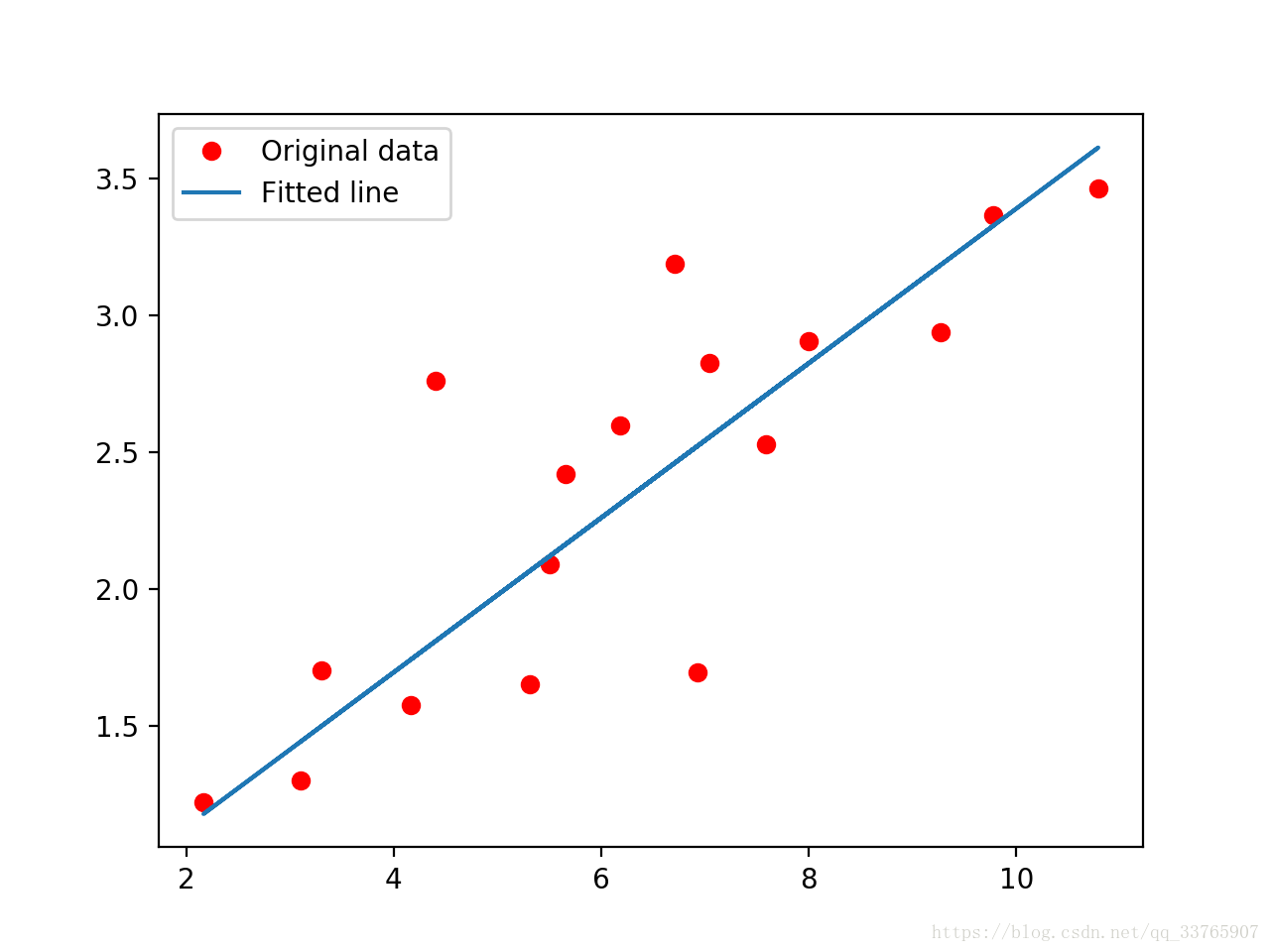
        plt.plot(train_X, train_Y, 'ro', label='Original data')
        plt.plot(train_X, sess.run(W) * train_X + sess.run(b), label='Fitted line')
        plt.legend()
        plt.show()

        # 测试数据集
        test_X = np.array([6.83, 4.668, 8.9, 7.91, 5.7, 8.7, 3.1, 2.1])
        test_Y = np.array([1.84, 2.273, 3.2, 2.831, 2.92, 3.24, 1.35, 1.03])

        print("Testing:")
        test_cost = sess.run(tf.reduce_sum(tf.pow(pred - Y, 2)) / (2 * test_X.shape[0]), feed_dict={X: test_X, Y: test_Y})
        print('Test cost =', test_cost)

        plt.plot(test_X, test_Y, 'bo', label='Testing data')
        plt.plot(train_X, sess.run(W) * train_X + sess.run(b), label='Fitted line')
        plt.legend()
        plt.show()

'''
output:
Epoch: 0050 cost= 0.077636465 W= 0.26401895 b= 0.6976915
Epoch: 0100 cost= 0.07756074 W= 0.263161 b= 0.70386344
Epoch: 0150 cost= 0.077493824 W= 0.262354 b= 0.7096687
Epoch: 0200 cost= 0.0774347 W= 0.261595 b= 0.7151288
Epoch: 0250 cost= 0.07738245 W= 0.26088107 b= 0.7202646
Epoch: 0300 cost= 0.07733631 W= 0.2602098 b= 0.72509426
Epoch: 0350 cost= 0.07729554 W= 0.25957844 b= 0.72963667
Epoch: 0400 cost= 0.077259526 W= 0.25898442 b= 0.7339096
Epoch: 0450 cost= 0.077227704 W= 0.25842583 b= 0.737928
Epoch: 0500 cost= 0.07719962 W= 0.2579005 b= 0.74170756
Epoch: 0550 cost= 0.077174835 W= 0.25740623 b= 0.74526274
Epoch: 0600 cost= 0.07715293 W= 0.25694156 b= 0.74860555
Epoch: 0650 cost= 0.07713358 W= 0.25650442 b= 0.7517508
Epoch: 0700 cost= 0.07711652 W= 0.2560933 b= 0.75470823
Epoch: 0750 cost= 0.077101454 W= 0.25570652 b= 0.7574905
Epoch: 0800 cost= 0.077088185 W= 0.25534278 b= 0.7601071
Epoch: 0850 cost= 0.07707646 W= 0.2550008 b= 0.76256734
Epoch: 0900 cost= 0.0770661 W= 0.25467893 b= 0.76488304
Epoch: 0950 cost= 0.07705698 W= 0.25437647 b= 0.76705915
Epoch: 1000 cost= 0.077048935 W= 0.2540919 b= 0.7691065
Optimization finished!
Training cost= 0.0019394646 W= 0.2540919 b= 0.7691065
'''
TensorFlow_线性回归实现

数据集和前面一篇一样。

猜你喜欢
