机器学习算法--朴素贝叶斯实践

1.贝叶斯理论

贝叶斯决策的核心：选择具有最高概率的决策

条件概率：

   

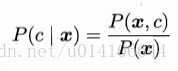
若P(c1|x)>P(c2|x)，则说明样本x应该属于c1类，直接对于P(c|x)不好求解，通过贝叶斯准则变换，转换为P(C),P(x|c)来求解

x=(x1,x2...xd)一般是一个d维特征向量，其联合分布难以计算，这里进行朴素贝叶斯假设，属性独立性假设，即每个属性对于分类结果的作用是独立的，因此P(x|c)=P(x1|c)*P(x2|c)....P(xd|c);分别计算训练集中每种类别的概率以及在具体的一类中各种属性特征的概率。

2.文本分类

判断一个文本的类型   c={侮辱性，非侮辱性}

样本的特征向量x为词汇表  表示该样本是否出现该词，1出现  0不出现

2.1 从文本中构建特征向量

处理训练文本，统计所有词转换成set集合，输出词汇表

def createVocabList(dataSet):
    vocabSet = set([])  #create empty set
    for document in dataSet:
        vocabSet = vocabSet | set(document) #union of the two sets
    return list(vocabSet)

根据词汇表以及样本文档，输出词汇向量x，其中1代表文档中出现该词  0代表没有出现该词

def setOfWords2Vec(vocabList, inputSet):
	#返回词汇向量和词向量长度一样
    returnVec = [0]*len(vocabList)
    for word in inputSet:
        if word in vocabList:
			#若出现则将对应词向量的位置置1
            returnVec[vocabList.index(word)] = 1
        else: print "the word: %s is not in my Vocabulary!" % word
    return returnVec

2.2从词向量计算概率

由P(ci|w) = P(ci,w)/P(w)=P(w|ci)*P(ci)/P(w)，其中w=(w1,w2....wn)为特征向量，假设个属性独立则有：

P(w|ci) = P(w1|ci)*P(w2|ci)....P(wn|ci);

即给定训练数据，首先计算各种类别ci的比重，对于具体的ci,计算其各个特征属性出现的概率P(wi|ci).

P(wi|ci)第ci类中属性wi所占的比重，P(wi|ci)=Dwici/Dci 

进行拉普拉斯平滑有 P(wi\ci)=(Dwici+1)/Dci+Ni.

为了防止小数相乘溢出取对数 

log(P(w|ci)*P(ci))=log(p(w1|ci))+log(p(w2|ci))+....+log(p(wn|ci))+log(p(ci))

def trainNB0(trainMatrix,trainCategory):
    #文档数量
    numTrainDocs = len(trainMatrix)
	#特征向量的维数
    numWords = len(trainMatrix[0])
	#trainCategory=1表示侮辱性文档  计算其概率
    pAbusive = sum(trainCategory)/float(numTrainDocs)
	#进行拉普拉斯平滑
    p0Num = ones(numWords); p1Num = ones(numWords)      #change to ones() 
    p0Denom = 2.0; p1Denom = 2.0                        #change to 2.0
    for i in range(numTrainDocs):
		#如果是侮辱性文档
        if trainCategory[i] == 1:
			#由于trainMatrix=1表示单词存在 因此同时进行所有侮辱性词汇数量的更新
            p1Num += trainMatrix[i]
			#侮辱性词汇总数量
            p1Denom += sum(trainMatrix[i])
        else:
            p0Num += trainMatrix[i]
            p0Denom += sum(trainMatrix[i])
	#进行对数运算，防止小数溢出  每个类别下各个特征向量的条件概率
    p1Vect = log(p1Num/p1Denom)          #change to log()
    p0Vect = log(p0Num/p0Denom)          #change to log()
    return p0Vect,p1Vect,pAbusive

输入为训练特征向量矩阵以及对应的类别信息矩阵  输出为各个类别下的各特征向量的条件概率以及各类别的概率，这里只输出侮辱性概率。

分类函数如下所示：

def classifyNB(vec2Classify, p0Vec, p1Vec, pClass1):
	#矩阵对应位置相乘  计算条件概率值
    p1 = sum(vec2Classify * p1Vec) + log(pClass1)    #element-wise mult
    p0 = sum(vec2Classify * p0Vec) + log(1.0 - pClass1)
    if p1 > p0:
        return 1
    else: 
        return 0

vec2Classify是待分类的特征向量。

3.测试

首先处理训练样本，确定特征向量W(w1,w2...wn)（文本中所有词集合），将训练样本转换为样本特征向量W=(w1,w2...wn)其中wi=1表示该词出现wi=0表示该词没有出现。根据训练样本类别信息C={c1,c2...cn}，确定各个类别的比重。对于每一类别，分析各种特征属性wi下的各自占比，根据NBC假设，P(C|W)=(P(C)*P(w1|C)*P(w2|C)...P(wn|C))/P(W),其中P(W)与具体的类别信息无关。计算P(Ci|W)即样本属于各种类别的概率，返回概率最大的类别作为样本的类别信息

def testingNB():
	#加载文档  类别向量
    listOPosts,listClasses = loadDataSet()
	#提取词向量
    myVocabList = createVocabList(listOPosts)
    trainMat=[] 
	#把文档转换为特征向量
    for postinDoc in listOPosts:
        trainMat.append(setOfWords2Vec(myVocabList, postinDoc))
	#训练贝叶斯返回类先验概率  以及P(X|C)先验概率向量
    p0V,p1V,pAb = trainNB0(array(trainMat),array(listClasses))
	#测试文档
    testEntry = ['love', 'my', 'dalmation']
	#测试样本向量
    thisDoc = array(setOfWords2Vec(myVocabList, testEntry))
	#分类结果
    print (testEntry,'classified as: ',classifyNB(thisDoc,p0V,p1V,pAb))
    testEntry = ['stupid', 'garbage']
    thisDoc = array(setOfWords2Vec(myVocabList, testEntry))
    print (testEntry,'classified as: ',classifyNB(thisDoc,p0V,p1V,pAb))

4.词袋模型与词集模型

以上特征向量中每一个元素取值为0或1，代表该词是否在该文档中出现，并没有考虑到各个单词在文档中出现的频率，词集模型。

词袋模型中，特征向量中记录每个词在文档中出现的次数。

def bagOfWords2VecMN(vocabList, inputSet):
    returnVec = [0]*len(vocabList)
    for word in inputSet:
		#如果该词出现过，则加一
        if word in vocabList:
            returnVec[vocabList.index(word)] += 1
    return returnVec

3.垃圾邮件过滤

文档内容---字符串列表--特征向量---NBC训练

将文档内容转化为字符串列表，一般使用正则表达式进行处理，使用非数字以及字母来分隔，返回分割后长度大于2的全部小写化的字符串

def textParse(bigString):    #input is big string, #output is word list
    import re
	#分隔  除字母和数字以外的任意字符串
    listOfTokens = re.split(r'\W*', bigString)
	#返回分割后的长度大于2转换为小写的字符
    return [tok.lower() for tok in listOfTokens if len(tok) > 2] 
    

文档一共有垃圾邮件26  非垃圾邮件26，一共52个样本，使用50个样本，随机产生10个用来测试，40个用来训练，多次训练和测试用来求出错误平均值：

def spamTest():
	#文档列表  类别列表      所有词列表
    docList=[]; classList = []; fullText =[]
    for i in range(1,26):
	    #非垃圾邮件训练样本
        wordList = textParse(open('email/spam/%d.txt' % i).read())
        docList.append(wordList)
        fullText.extend(wordList)
        classList.append(1)
		#垃圾邮件训练样本
        wordList = textParse(open('email/ham/%d.txt' % i).read())
        docList.append(wordList)
        fullText.extend(wordList)
        classList.append(0)
	#创建词向量
    vocabList = createVocabList(docList)#create vocabulary
	#训练集索引   测试集索引
    trainingSet = list(range(50)); testSet=[]           #create test set
	#50个样本随机产生10个测试集以及40个训练集
    for i in range(10):
        randIndex = int(random.uniform(0,len(trainingSet)))
        testSet.append(trainingSet[randIndex])
        del(trainingSet[randIndex])  
    trainMat=[]; trainClasses = []
	#用训练集进行训练
    for docIndex in trainingSet:#train the classifier (get probs) trainNB0
        trainMat.append(bagOfWords2VecMN(vocabList, docList[docIndex]))
        trainClasses.append(classList[docIndex])
    p0V,p1V,pSpam = trainNB0(array(trainMat),array(trainClasses))
    errorCount = 0
	#用测试集进行测试
    for docIndex in testSet:        #classify the remaining items
        wordVector = bagOfWords2VecMN(vocabList, docList[docIndex])
        if classifyNB(array(wordVector),p0V,p1V,pSpam) != classList[docIndex]:
            errorCount += 1
            print ("classification error",docList[docIndex])
    print ('the error rate is: ',float(errorCount)/len(testSet))
    #return vocabList,fullText

关于模型的评估：

1.留出法。将样本分为训练集S以及测试集T，用S来训练用T来测试，来对泛化误差进行评估

2.交叉验证。将数据集D划分为K个互斥的子集D1,D2...Dk   每次使用其中k-1个子集训练，剩余一个测试。进行k次，取平均值。

3.自助法。数据集D中m个元素  通过随机采样获得元素复制到D`,该元素继续在D中被采样，进行m次，即可得到数据集D`

样本进行m次采用，始终不被采到的概率是：

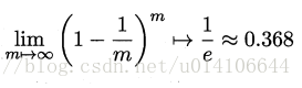
即测试集的比重约为0.36.

4.RSS分类器

根据两个不同RSS的用词不同，来对文档进行RSS分类

def calcMostFreq(vocabList,fullText,num):
    import operator
	#字典  key词   value次数
    freqDict = {}
    for token in vocabList:
        freqDict[token]=fullText.count(token)
    sortedFreq = sorted(freqDict.items(), key=operator.itemgetter(1), reverse=True)
    #返回出现频率最高的30个词	
    return sortedFreq[:num]       

def localWords(feed1,feed0,num):
    import feedparser
    docList=[]; classList = []; fullText =[]
    minLen = min(len(feed1['entries']),len(feed0['entries']))
    for i in range(minLen):
        wordList = textParse(feed1['entries'][i]['summary'])
        docList.append(wordList)
        fullText.extend(wordList)
        classList.append(1) #NY is class 1
        wordList = textParse(feed0['entries'][i]['summary'])
        docList.append(wordList)
        fullText.extend(wordList)
        classList.append(0)
	#创建词向量
    vocabList = createVocabList(docList)#create vocabulary
	#计算频率最高的30词
    top30Words = calcMostFreq(vocabList,fullText,num)   #remove top 30 words
	#去除掉频率最高的30词
    for pairW in top30Words:
        if pairW[0] in vocabList: vocabList.remove(pairW[0])
	#训练集  测试集随机10
    trainingSet = list(range(2*minLen)); testSet=[]           #create test set
    for i in range(10):
        randIndex = int(random.uniform(0,len(trainingSet)))
        testSet.append(trainingSet[randIndex])
        del(trainingSet[randIndex])  
    trainMat=[]; trainClasses = []
	#训练集进行训练
    for docIndex in trainingSet:#train the classifier (get probs) trainNB0
        trainMat.append(bagOfWords2VecMN(vocabList, docList[docIndex]))
        trainClasses.append(classList[docIndex])
    p0V,p1V,pSpam = trainNB0(array(trainMat),array(trainClasses))
    errorCount = 0
	#测试集进行测试
    for docIndex in testSet:        #classify the remaining items
        wordVector = bagOfWords2VecMN(vocabList, docList[docIndex])
        if classifyNB(array(wordVector),p0V,p1V,pSpam) != classList[docIndex]:
            errorCount += 1
    print ('the error rate is: ',float(errorCount)/len(testSet))
    return vocabList,p0V,p1V

        分别加载两个不同RSS源的数据，类别属性为1,0.  由于文档中存在大量的停用词，即这些词语在任何文档中都可能大量出现，并没有区分性，因此可以去除掉这些高频词来优化分类模型。获取所有样本数据，计算词向量，随机选择10个测试集，用训练集来训练模型，用测试集来测试模型。可以通过改变取出高频词的个数来优化模型的性能。

 ny = feedparser.parse('http://www.nasa.gov/rss/dyn/image_of_the_day.rss')

 sf  = feedparser.parse('http://sports.yahoo.com/nba/teams/hou/rss.xml')

测试结果如下：

显示地域相关用词

def getTopWords(ny,sf,num):
    import operator
    vocabList,p0V,p1V=localWords(ny,sf,num)
    topNY=[]; topSF=[]
    for i in range(len(p0V)):
        if p0V[i] > -6.0 : topSF.append((vocabList[i],p0V[i]))
        if p1V[i] > -6.0 : topNY.append((vocabList[i],p1V[i]))
    sortedSF = sorted(topSF, key=lambda pair: pair[1], reverse=True)
    print ("SF**SF**SF**SF**SF**SF**SF**SF**SF**SF**SF**SF**SF**SF**SF**SF**")
    for item in sortedSF:
        print (item[0])
    sortedNY = sorted(topNY, key=lambda pair: pair[1], reverse=True)
    print ("NY**NY**NY**NY**NY**NY**NY**NY**NY**NY**NY**NY**NY**NY**NY**NY**")
    for item in sortedNY:
        print (item[0])