Matplotlib python 学习笔记3

课程地址：网易云课堂
https://study.163.com/course/courseMain.htm?courseId=1003240004
或者：
https://morvanzhou.github.io/tutorials/data-manipulation/plt/
莫烦大神的主页：
https://morvanzhou.github.io

以下代码全都在jupyter notebook中通过

# %matplotlib qt5
%matplotlib inline
import matplotlib.pyplot as plt

plt.figure()

#均匀图中图
plt.subplot(2,2,1)   # 把figure分成两行两列，在第一个位置画图
plt.plot([0,1],[0,1])
plt.subplot(2,2,2)   # 把figure分成两行两列，在第2个位置画图
plt.plot([0,1],[0,2])
plt.subplot(2,2,3)   # 把figure分成两行两列，在第3个位置画图
# plt.subplot(223)  #智能识别
plt.plot([0,1],[0,3])
plt.subplot(2,2,4)   # 把figure分成两行两列，在第4个位置画图
# plt.subplot(224)
plt.plot([0,1],[0,4])

# #不均匀图中图
# plt.subplot(2,1,1)  #将整个图像窗口分为2行1列, 当前位置为1.
# plt.plot([0,1],[0,1])
# plt.subplot(2,3,4)  #将整个图像窗口分为2行3列, 当前位置为4
# plt.plot([0,1],[0,2])
# plt.subplot(235)   #将整个图像窗口分为2行3列, 当前位置为5
# plt.plot([0,1],[0,3])
# plt.subplot(236)  #将整个图像窗口分为2行3列, 当前位置为6
# plt.plot([0,1],[0,4])

plt.show()

import matplotlib.pyplot as plt
import matplotlib.gridspec as gridspec

# # method 1 : subplot2grid
# ######################
# plt.figure()
# ax1 = plt.subplot2grid((3,3),(0,0),colspan=3,rowspan=1)
# #将figure划分为3行3列，在(0,0)位置开始画图，跨度为1行3列
# ax1.plot([1,2],[1,2])
# ax1.set_title('ax1_title')
# #plt.xlim之类都变成ax1.set_
# ax2 = plt.subplot2grid((3,3),(1,0),colspan=2)
# # ax2 = plt.subplot2grid((3,3),(1,0),colspan=2,rowspan=1)    #  和上句效果一样
# ax3 = plt.subplot2grid((3,3),(1,2),rowspan=2)
# ax4 = plt.subplot2grid((3,3),(2,0))
# ax5 = plt.subplot2grid((3,3),(2,1))

# ax2.set_title('ax2_title')
# ax3.set_title('ax3_title')
# ax4.set_title('ax4_title')
# ax5.set_title('ax5_title')   


# method 2 : gridspec
######################
#import matplotlib.gridspec as gridspec   #需要import这个,其它两种方法不需要
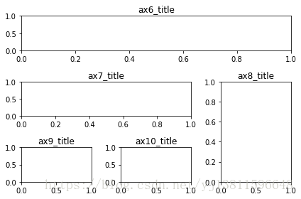
plt.figure()
gs = gridspec.GridSpec(3,3)
ax6 = plt.subplot(gs[0, :])   #占据第0行，占据所有列
ax7 = plt.subplot(gs[1, :2])  #占据第1行，占据0，1列
ax8 = plt.subplot(gs[1:, 2])  #占据第1，2行，占据第2列
ax9 = plt.subplot(gs[-1, 0]) #占据最后一行，占据第0列
ax10 = plt.subplot(gs[-1, -2]) #占据最后一行，占据倒数第2列

ax6.set_title('ax6_title')
ax7.set_title('ax7_title')
ax8.set_title('ax8_title')
ax9.set_title('ax9_title')
ax10.set_title('ax10_title')   


# # method 3 : easy to define structure
# ######################
# f,((ax11,ax12),(ax21,ax22)) = plt.subplots(2,2,sharex=True,sharey=True)
# ax11.scatter([1,2],[1,2])

# ax11.set_title('ax11_title')
# ax12.set_title('ax12_title')
# ax21.set_title('ax21_title')
# ax22.set_title('ax22_title')
# #其实这种方法也是有几个图就有几个坐标轴，但看上去好像只有一个坐标轴一样

plt.tight_layout()  #表示紧凑显示图像
plt.show()   #表示显示图像

# %matplotlib inline
# %matplotlib qt5

# 导入pyplot模块
import matplotlib.pyplot as plt

# 初始化figure
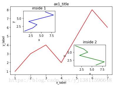
fig = plt.figure()

# 创建数据
x = [1, 2, 3, 4, 5, 6, 7]
y = [1, 3, 4, 2, 5, 8, 6]

#首先确定大图左下角的位置以及宽高：
left, bottom, width, height = 0.1, 0.1, 0.8, 0.8     
#注意，4个值都是占整个figure坐标系的百分比。
#在这里，假设figure的大小是10x10，那么大图就被包含在由(1, 1)开始，宽8，高8的坐标系内。
#显示在gui里才能看出来，显示在控制台看不出来

ax1 = fig.add_axes([left, bottom, width, height])
ax1.plot(x, y, 'r')
ax1.set_xlabel('x_label')
ax1.set_ylabel('y_label')
ax1.set_title('ax1_title')

#接着，我们来绘制左上角的小图，步骤和绘制大图一样，注意坐标系位置和大小的改变：
left, bottom, width, height = 0.2, 0.6, 0.25, 0.25
ax2 = fig.add_axes([left, bottom, width, height])
ax2.plot(y, x, 'b')   #把x,y反过来图像就不一样了
ax2.set_xlabel('x')
ax2.set_ylabel('y')
ax2.set_title('inside 1')


#最后，我们来绘制右下角的小图。这里我们采用一种更简单方法，即直接往plt里添加新的坐标系：
plt.axes([0.6, 0.2, 0.25, 0.25])
plt.plot(y[::-1], x, 'g')   # 注意对y进行了逆序处理
plt.xlabel('x')
plt.ylabel('y')
plt.title('inside 2')


plt.show()

import matplotlib.pyplot as plt
import numpy as np

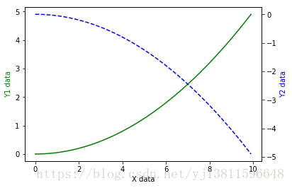
x = np.arange(0, 10, 0.1)

y1 = 0.05 * x**2

y2 = -1 * y1

fig, ax1 = plt.subplots()
ax2 = ax1.twinx()    #对ax1调用twinx()方法，生成如同镜面效果后的ax2

ax1.plot(x, y1, 'g-')   # green, solid line
ax1.set_xlabel('X data')
ax1.set_ylabel('Y1 data', color='g')

ax2.plot(x, y2, 'b--') # blue
ax2.set_ylabel('Y2 data', color='b')



plt.show()

%matplotlib qt5

from matplotlib import pyplot as plt
from matplotlib import animation
import numpy as np

fig, ax = plt.subplots()

x = np.arange(0, 2*np.pi, 0.01)   #我们的数据是一个0~2π内的正弦曲线：
line, = ax.plot(x, np.sin(x))   #选择列表的第一位？

def animate(i):
    line.set_ydata(np.sin(x + i/10.0))
    return line,

def init():
    line.set_ydata(np.sin(x))
    return line,


# 接下来，我们调用FuncAnimation函数生成动画。参数说明：

# fig 进行动画绘制的figure
# func 自定义动画函数，即传入刚定义的函数animate
# frames 动画长度，一次循环包含的帧数
# init_func 自定义开始帧，即传入刚定义的函数init
# interval 更新频率，以ms计
# blit 选择更新所有点，还是仅更新产生变化的点。应选择True，但mac用户请选择False，否则无法显示动画

ani = animation.FuncAnimation(fig=fig,
                              func=animate,
                              frames=100,
                              init_func=init,
                              interval=20,
                              blit=False)


plt.show()

# ani.save('basic_animation.mp4', fps=30, extra_args=['-vcodec', 'libx264'])
# 保存不了，MovieWriter ffmpeg unavailable.