Sklearn-LogisticRegression逻辑回归(有处理样本不均衡时设置参数的方法)

版权声明：本文为博主原创文章，未经博主允许不得转载。 https://blog.csdn.net/CherDW/article/details/54891073

1. 逻辑回归：

可以做概率预测，也可用于分类，仅能用于线性问题。通过计算真实值与预测值的概率，然后变换成损失函数，求损失函数最小值来计算模型参数，从而得出模型。

1. sklearn.linear_model.LogisticRegression官方API：

官方API：http://scikit-learn.org/stable/modules/generated/sklearn.linear_model.LogisticRegression.html

classsklearn.linear_model.LogisticRegression(penalty='l2', dual=False, tol=0.0001, C=1.0,fit_intercept=True, intercept_scaling=1, class_weight=None, random_state=None,solver='liblinear', max_iter=100, multi_class='ovr', verbose=0,warm_start=False, n_jobs=1)

1. 参数解读

• 正则化选择参数（惩罚项的种类）

penalty: str,‘l1’or ‘l2’,default: ‘l2’

Usedto specify the norm used in the penalization. The ‘newton-cg’, ‘sag’ and‘lbfgs’ solvers support only l2 penalties.

• LogisticRegression默认带了正则化项。penalty参数可选择的值为"l1"和"l2".分别对应L1的正则化和L2的正则化，默认是L2的正则化。
• 在调参时如果我们主要的目的只是为了解决过拟合，一般penalty选择L2正则化就够了。但是如果选择L2正则化发现还是过拟合，即预测效果差的时候，就可以考虑L1正则化。另外，如果模型的特征非常多，我们希望一些不重要的特征系数归零，从而让模型系数稀疏化的话，也可以使用L1正则化。
• penalty参数的选择会影响我们损失函数优化算法的选择。即参数solver的选择，如果是L2正则化，那么4种可选的算法{‘newton-cg’, ‘lbfgs’, ‘liblinear’, ‘sag’}都可以选择。但是如果penalty是L1正则化的话，就只能选择‘liblinear’了。这是因为L1正则化的损失函数不是连续可导的，而{‘newton-cg’, ‘lbfgs’,‘sag’}这三种优化算法时都需要损失函数的一阶或者二阶连续导数。而‘liblinear’并没有这个依赖。

• dual: bool,default: False

Dualor primal formulation. Dual formulation is only implemented for l2 penalty withliblinear solver. Preferdual=False whenn_samples > n_features.

• 对偶或者原始方法。Dual只适用于正则化相为l2 liblinear的情况，通常样本数大于特征数的情况下，默认为False。

• C: float,default: 1.0

Inverseof regularization strength; must be a positive float. Like in support vectormachines, smaller values specify stronger regularization.

• C为正则化系数λ的倒数，通常默认为1

• fit_intercept: bool,default: True

Specifiesif a constant (a.k.a. bias or intercept) should be added to the decisionfunction.

• 是否存在截距，默认存在

• intercept_scaling: float,default 1.

Usefulonly when the solver ‘liblinear’ is used and self.fit_intercept is set to True.In this case, x becomes [x, self.intercept_scaling], i.e. a “synthetic” featurewith constant value equal to intercept_scaling is appended to the instancevector. The intercept becomes intercept_scaling * synthetic_feature_weight.

Note!the synthetic feature weight is subject to l1/l2 regularization as all otherfeatures. To lessen the effect of regularization on synthetic feature weight(and therefore on the intercept) intercept_scaling has to be increased.

仅在正则化项为"liblinear"，且fit_intercept设置为True时有用。

• 优化算法选择参数

solver

{‘newton-cg’, ‘lbfgs’, ‘liblinear’, ‘sag’},default: ‘liblinear’

Algorithmto use in the optimization problem.

Forsmall datasets, ‘liblinear’ is a good choice, whereas ‘sag’ is

fasterfor large ones.

Formulticlass problems, only ‘newton-cg’, ‘sag’ and ‘lbfgs’ handle

multinomialloss; ‘liblinear’ is limited to one-versus-rest schemes.

‘newton-cg’,‘lbfgs’ and ‘sag’ only handle L2 penalty.

Notethat ‘sag’ fast convergence is only guaranteed on features with approximatelythe same scale. You can preprocess the data with a scaler fromsklearn.preprocessing.

Newin version 0.17: Stochastic Average Gradient descent solver.

• solver参数决定了我们对逻辑回归损失函数的优化方法，有四种算法可以选择，分别是：

a) liblinear：使用了开源的liblinear库实现，内部使用了坐标轴下降法来迭代优化损失函数。

b) lbfgs：拟牛顿法的一种，利用损失函数二阶导数矩阵即海森矩阵来迭代优化损失函数。

c) newton-cg：也是牛顿法家族的一种，利用损失函数二阶导数矩阵即海森矩阵来迭代优化损失函数。

d) sag：即随机平均梯度下降，是梯度下降法的变种，和普通梯度下降法的区别是每次迭代仅仅用一部分的样本来计算梯度，适合于样本数据多的时候。

• 从上面的描述可以看出，newton-cg, lbfgs和sag这三种优化算法时都需要损失函数的一阶或者二阶连续导数，因此不能用于没有连续导数的L1正则化，只能用于L2正则化。而liblinear通吃L1正则化和L2正则化。
• 同时，sag每次仅仅使用了部分样本进行梯度迭代，所以当样本量少的时候不要选择它，而如果样本量非常大，比如大于10万，sag是第一选择。但是sag不能用于L1正则化，所以当你有大量的样本，又需要L1正则化的话就要自己做取舍了。要么通过对样本采样来降低样本量，要么回到L2正则化。
• 从上面的描述，大家可能觉得，既然newton-cg, lbfgs和sag这么多限制，如果不是大样本，我们选择liblinear不就行了嘛！错，因为liblinear也有自己的弱点！我们知道，逻辑回归有二元逻辑回归和多元逻辑回归。对于多元逻辑回归常见的有one-vs-rest(OvR)和many-vs-many(MvM)两种。而MvM一般比OvR分类相对准确一些。郁闷的是liblinear只支持OvR，不支持MvM，这样如果我们需要相对精确的多元逻辑回归时，就不能选择liblinear了。也意味着如果我们需要相对精确的多元逻辑回归不能使用L1正则化了。

• 总结几种优化算法适用情况：

L1	liblinear	liblinear适用于小数据集；如果选择L2正则化发现还是过拟合，即预测效果差的时候，就可以考虑L1正则化；如果模型的特征非常多，希望一些不重要的特征系数归零，从而让模型系数稀疏化的话，也可以使用L1正则化。
L2	liblinear	libniear只支持多元逻辑回归的OvR，不支持MvM，但MVM相对精确。
L2	lbfgs/newton-cg/sag	较大数据集，支持one-vs-rest(OvR)和many-vs-many(MvM)两种多元逻辑回归。
L2	sag	如果样本量非常大，比如大于10万，sag是第一选择；但不能用于L1正则化。

　　　　具体OvR和MvM有什么不同下一节讲。

• 分类方式选择参数：

multi_class: str,{‘ovr’, ‘multinomial’},default:‘ovr’

Multiclassoption can be either ‘ovr’ or ‘multinomial’. If the option chosen is ‘ovr’,then a binary problem is fit for each label. Else the loss minimised is themultinomial loss fit across the entire probability distribution. Works only forthe ‘newton-cg’, ‘sag’ and ‘lbfgs’ solver.

Newin version 0.18: Stochastic Average Gradient descent solver for ‘multinomial’case.

• ovr即前面提到的one-vs-rest(OvR)，而multinomial即前面提到的many-vs-many(MvM)。如果是二元逻辑回归，ovr和multinomial并没有任何区别，区别主要在多元逻辑回归上。
• OvR和MvM有什么不同？

        OvR的思想很简单，无论你是多少元逻辑回归，我们都可以看做二元逻辑回归。具体做法是，对于第K类的分类决策，我们把所有第K类的样本作为正例，除了第K类样本以外的所有样本都作为负例，然后在上面做二元逻辑回归，得到第K类的分类模型。其他类的分类模型获得以此类推。

        而MvM则相对复杂，这里举MvM的特例one-vs-one(OvO)作讲解。如果模型有T类，我们每次在所有的T类样本里面选择两类样本出来，不妨记为T1类和T2类，把所有的输出为T1和T2的样本放在一起，把T1作为正例，T2作为负例，进行二元逻辑回归，得到模型参数。我们一共需要T(T-1)/2次分类。

        可以看出OvR相对简单，但分类效果相对略差（这里指大多数样本分布情况，某些样本分布下OvR可能更好）。而MvM分类相对精确，但是分类速度没有OvR快。如果选择了ovr，则4种损失函数的优化方法liblinear，newton-cg,lbfgs和sag都可以选择。但是如果选择了multinomial,则只能选择newton-cg, lbfgs和sag了。

• 类型权重参数：（考虑误分类代价敏感、分类类型不平衡的问题）

class_weight: dictor ‘balanced’,default: None

Weightsassociated with classes in the form {class_label: weight}. If not given, allclasses are supposed to have weight one.

The“balanced” mode uses the values of y to automatically adjust weights inverselyproportional to class frequencies in the input data as n_samples / (n_classes *np.bincount(y)).

Notethat these weights will be multiplied with sample_weight (passed through thefit method) if sample_weight is specified.

Newin version 0.17: class_weight=’balanced’ instead of deprecatedclass_weight=’auto’.

• class_weight参数用于标示分类模型中各种类型的权重，可以不输入，即不考虑权重，或者说所有类型的权重一样。如果选择输入的话，可以选择balanced让类库自己计算类型权重，或者我们自己输入各个类型的权重，比如对于0,1的二元模型，我们可以定义class_weight={0:0.9, 1:0.1}，这样类型0的权重为90%，而类型1的权重为10%。
• 如果class_weight选择balanced，那么类库会根据训练样本量来计算权重。某种类型样本量越多，则权重越低，样本量越少，则权重越高。当class_weight为balanced时，类权重计算方法如下：n_samples / (n_classes * np.bincount(y))

n_samples为样本数，n_classes为类别数量，np.bincount(y)会输出每个类的样本数，例如y=[1,0,0,1,1],则np.bincount(y)=[2,3]

• 那么class_weight有什么作用呢？

       在分类模型中，我们经常会遇到两类问题：

        第一种是误分类的代价很高。比如对合法用户和非法用户进行分类，将非法用户分类为合法用户的代价很高，我们宁愿将合法用户分类为非法用户，这时可以人工再甄别，但是却不愿将非法用户分类为合法用户。这时，我们可以适当提高非法用户的权重。

       第二种是样本是高度失衡的，比如我们有合法用户和非法用户的二元样本数据10000条，里面合法用户有9995条，非法用户只有5条，如果我们不考虑权重，则我们可以将所有的测试集都预测为合法用户，这样预测准确率理论上有99.95%，但是却没有任何意义。这时，我们可以选择balanced，让类库自动提高非法用户样本的权重。

       提高了某种分类的权重，相比不考虑权重，会有更多的样本分类划分到高权重的类别，从而可以解决上面两类问题。

       当然，对于第二种样本失衡的情况，我们还可以考虑用下一节讲到的样本权重参数：sample_weight，而不使用class_weight。sample_weight在下一节讲。

• 样本权重参数：

sample_weight（fit函数参数）

• 当样本是高度失衡的，导致样本不是总体样本的无偏估计，从而可能导致我们的模型预测能力下降。遇到这种情况，我们可以通过调节样本权重来尝试解决这个问题。调节样本权重的方法有两种，第一种是在class_weight使用balanced。第二种是在调用fit函数时，通过sample_weight来自己调节每个样本权重。在scikit-learn做逻辑回归时，如果上面两种方法都用到了，那么样本的真正权重是class_weight*sample_weight.

• max_iter: int,default: 100

Usefulonly for the newton-cg, sag and lbfgs solvers. Maximum number of iterationstaken for the solvers to converge.

• 仅在正则化优化算法为newton-cg, sag and lbfgs才有用，算法收敛的最大迭代次数。

• random_state: int seed, RandomState instance,default: None

The seed of the pseudo random number generator touse when shuffling the data. Used only in solvers ‘sag’ and ‘liblinear’.

• 随机数种子，默认为无，仅在正则化优化算法为sag,liblinear时有用。

• tol :float,default: 1e-4

Tolerance for stopping criteria.迭代终止判据的误差范围。

• verbose: int, default: 0

Forthe liblinear and lbfgs solvers set verbose to any positive number forverbosity.

• 日志冗长度int：冗长度；0：不输出训练过程；1：偶尔输出；>1：对每个子模型都输出

• warm_start: bool,default: False

Whenset to True, reuse the solution of the previous call to fit as initialization,otherwise, just erase the previous solution. Useless for liblinear solver.

Newin version 0.17: warm_start to support lbfgs, newton-cg, sag solvers.

• 是否热启动，如果是，则下一次训练是以追加树的形式进行（重新使用上一次的调用作为初始化），bool：热启动，False：默认值

• n_jobs: int, default: 1

Numberof CPU cores used during the cross-validation loop. If given a value of -1, allcores are used.

• 并行数，int：个数；-1：跟CPU核数一致；1:默认值

1. LogisticRegression类中的方法

LogisticRegression类中的方法有如下几种，常用的是fit和predict

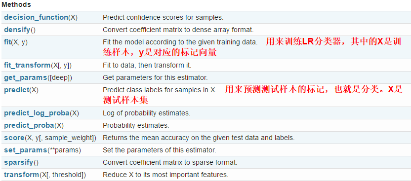
• fit(X, y, sample_weight=None)

Fitthe model according to the given training data.

Parameters:        

X: {array-like, sparse matrix}, shape (n_samples, n_features)

Trainingvector, where n_samples is the number of samples and n_features is the numberof features.

y: array-like, shape (n_samples,)

Targetvector relative to X.

sample_weight:array-like, shape (n_samples,)optional

Arrayof weights that are assigned to individual samples. If not provided, then eachsample is given unit weight.

Newin version 0.17: sample_weight support to LogisticRegression.

Returns:        

self: object

Returnsself.

• 拟合模型，用来训练LR分类器，其中X是训练样本，y是对应的标记向量

• fit_transform(X, y=None, **fit_params)

Fitto data, then transform it.

Fitstransformer to X and y with optional parameters fit_params and returns atransformed version of X.

Parameters:        

X: numpy array of shape [n_samples, n_features]

Trainingset.

y: numpy array of shape [n_samples]

Targetvalues.

Returns:        

X_new: numpy array of shape [n_samples, n_features_new]

Transformedarray.

• fit与transform的结合，先fit后transform

• transform(*args, **kwargs)

DEPRECATED:Support to use estimators as feature selectors will be removed in version 0.19.Use SelectFromModel instead.

ReduceX to its most important features.

Usescoef_ or feature_importances_ to determine the most important features. Formodels with a coef_ for each class, the absolute sum over the classes is used.

Parameters:        

X: array or scipy sparse matrix of shape [n_samples, n_features]

Theinput samples.

Threshold:string, float or None, optional (default=None)

The threshold value to use for featureselection. Features whose importance is greater or equal are kept while theothers are discarded.If “median” (resp. “mean”), then the thresholdvalue is the median (resp. the mean) of the feature importances. A scalingfactor (e.g., “1.25*mean”) may also be used. If None and if available, theobject attribute threshold is used. Otherwise,“mean” is used by default.

Returns:        

X_r: array of shape [n_samples, n_selected_features]

Theinput samples with only the selected features.

•  默认使用特征重要性平均值作为阈值对特征进行筛选

• predict(X)[source]

Predictclass labels for samples in X.

Parameters:        

X: {array-like, sparse matrix}, shape = [n_samples, n_features]

Samples.

Returns:        

C: array, shape = [n_samples]

Predictedclass label per sample.

用来预测样本的标记，也就是分类，X是测试集

• predict_proba(X)

Probabilityestimates.

The returned estimates for all classes areordered by the label of classes.

Fora multi_class problem, if multi_class is set to be “multinomial” the softmaxfunction is used to find the predicted probability of each class. Else use aone-vs-rest approach, i.e calculate the probability of each class assuming itto be positive using the logistic function. and normalize these values acrossall the classes.

Parameters:        

X :array-like, shape = [n_samples, n_features]

Returns:        

T :array-like, shape = [n_samples, n_classes]

Returns the probability of the sample foreach class in the model, where classes are ordered as they are inself.classes_.

• 输出分类概率。返回每种类别的概率，按照分类类别顺序给出。如果是多分类问题，multi_class="multinomial"，则会给出样本对于每种类别的概率。

1. 示例

1. #分开训练集、测试集

2. train= loan_data.iloc[0: 55596, :]

3. test= loan_data.iloc[55596:, :]

4. # 避免过拟合，采用交叉验证，验证集占训练集20%，固定随机种子（这里所用的数据都是在训练集上进行）

5. train_X,test_X, train_y, test_y = train_test_split(train,

6. target,

7. test_size = 0.2,

8. random_state = 0)

9. train_y= train_y['label']

10. test_y= test_y['label']

11. # 用Logistic回归建模

12. lr_model= LogisticRegression(C = 1.0,

13. penalty = 'l2')

14. lr_model.fit(train_X,train_y)

15. # 给出交叉验证集的预测结果，并输出评估的准确率、召回率、F1值

16. pred_test= lr_model.predict(test_X)

17. printclassification_report(test_y, pred_test)

18. # 输出测试集用户逾期还款概率，predict_proba会输出两个概率，即分别分类为‘0’和‘1’的概率，这里只取‘1’的概率

19. pred= lr_model.predict_proba(test)

20. result= pd.DataFrame(pred)

21. result.index= test.index

22. result.columns= ['0', 'probability']

23. result.drop('0',

24. axis = 1,

25. inplace = True)

26. printresult.head(5)

27. #输出结果

28. result.to_csv('result.csv')

 

--------------------- 本文来自 Cherzhoucheer 的CSDN 博客 ，全文地址请点击：https://blog.csdn.net/cherdw/article/details/54891073?utm_source=copy