以前都是用SPSS/EVIEWS等来做的,现在用Python来搞搞看,前后弄了一个星期,总算基本走通了。
基础库: pandas,numpy,scipy,matplotlib,statsmodels :
from __future__ import print_function
import pandas as pd
import numpy as np
from scipy import stats
import matplotlib.pyplot as plt
import statsmodels.api as sm
from statsmodels.graphics.api import qqplot
运行的时候会报错:Undefined variable from import:,不过好像不影响结果
1.数据:
dta=[10930,10318,10595,10972,7706,6756,9092,10551,9722,10913,11151,8186,6422,
6337,11649,11652,10310,12043,7937,6476,9662,9570,9981,9331,9449,6773,6304,9355,
10477,10148,10395,11261,8713,7299,10424,10795,11069,11602,11427,9095,7707,10767,
12136,12812,12006,12528,10329,7818,11719,11683,12603,11495,13670,11337,10232,
13261,13230,15535,16837,19598,14823,11622,19391,18177,19994,14723,15694,13248,
9543,12872,13101,15053,12619,13749,10228,9725,14729,12518,14564,15085,14722,
11999,9390,13481,14795,15845,15271,14686,11054,10395]
dta=np.array(dta,dtype=np.float) //这里要转下数据类型,不然运行会报错

dta=pd.Series(dta)
dta.index = pd.Index(sm.tsa.datetools.dates_from_range('2001','2090')) //应该是2090,不是2100
dta.plot(figsize=(12,8))
plt.show() // 在Scala IDE要输入这个命令才能显示图片
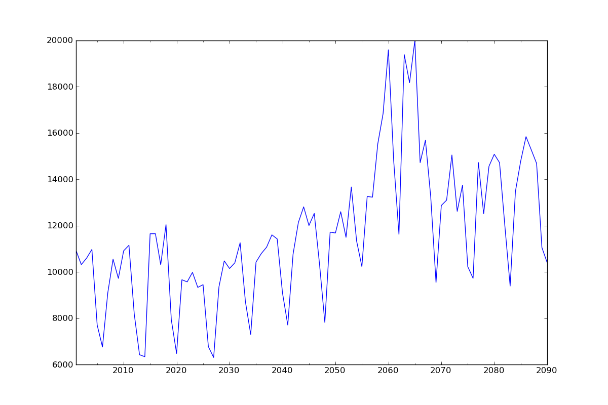
2.时间序列的差分d
ARIMA 模型对时间序列的要求是平稳型。因此,当你得到一个非平稳的时间序列时,首先要做的即是做时间序列的差分,直到得到一个平稳时间序列。如果你对时间序列做d次差分才能得到一个平稳序列,那么可以使用ARIMA(p,d,q)模型,其中d是差分次数。
fig = plt.figure(figsize=(12,8))
ax1= fig.add_subplot(111)
diff1 = dta.diff(1)
diff1.plot(ax=ax1)
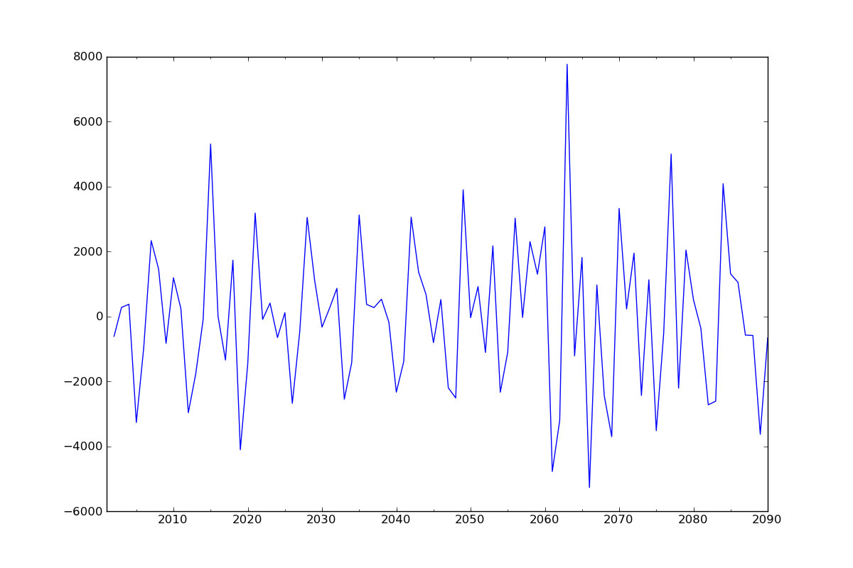
已经平稳,二阶效果也差不多,具体见原文
3.合适的p,q
现在我们已经得到一个平稳的时间序列,接来下就是选择合适的ARIMA模型,即ARIMA模型中合适的p,q 。
3.1 第一步我们要先检查平稳时间序列的自相关图和偏自相关图。
diff1= dta.diff(1)#我们已经知道要使用一阶差分的时间序列,之前判断差分的程序可以注释掉 //原文有错误应该是diff1= dta.diff(1),而非dta= dta.diff(1)
fig = plt.figure(figsize=(12,8))
ax1=fig.add_subplot(211)
fig = sm.graphics.tsa.plot_acf(dta,lags=40,ax=ax1)
ax2 = fig.add_subplot(212)
fig = sm.graphics.tsa.plot_pacf(dta,lags=40,ax=ax2)
其中lags 表示滞后的阶数,以上分别得到acf 图和pacf 图
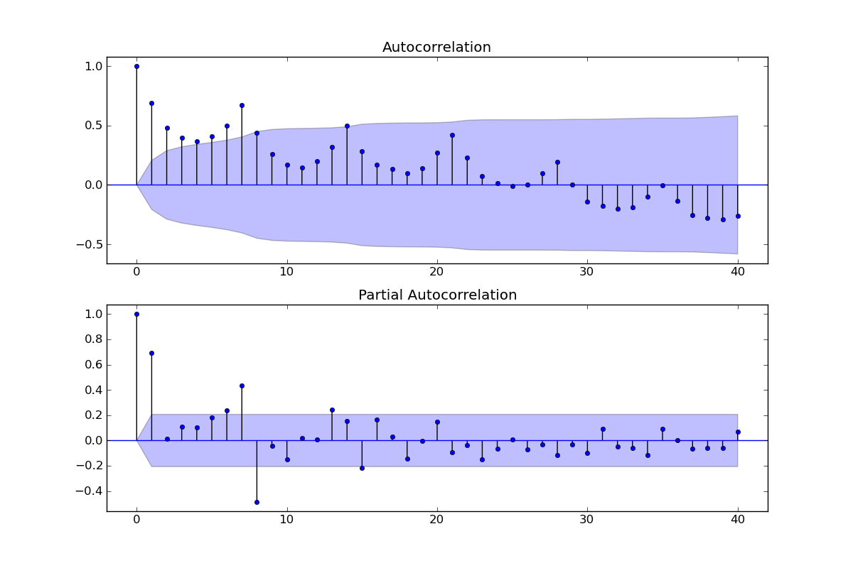
通过两图观察得到:
* 自相关图显示滞后有三个阶超出了置信边界;
* 偏相关图显示在滞后1至7阶(lags 1,2,…,7)时的偏自相关系数超出了置信边界,从lag 7之后偏自相关系数值缩小至0
3.2模型选择
根据上图,猜测有以下模型可以供选择:
1)ARMA(0,1)模型:即自相关图在滞后1阶之后缩小为0,且偏自相关缩小至0,则是一个阶数q=1的移动平均模型;
2.)ARMA(7,0)模型:即偏自相关图在滞后7阶之后缩小为0,且自相关缩小至0,则是一个阶层p=7的自回归模型; //原文错写为3
3.)ARMA(7,1)模型:即使得自相关和偏自相关都缩小至零。则是一个混合模型。
4) …还可以有其他供选择的模型 (实际上下文选了ARMA(8,0))
现在有以上这么多可供选择的模型,我们通常采用ARMA模型的AIC法则。我们知道:增加自由参数的数目提高了拟合的优良性,AIC鼓励数据拟合的优良性但是尽量避免出现过度拟合(Overfitting)的情况。所以优先考虑的模型应是AIC值最小的那一个。赤池信息准则的方法是寻找可以最好地解释数据但包含最少自由参数的模型。不仅仅包括AIC准则,目前选择模型常用如下准则:
* AIC=-2 ln(L) + 2 k 中文名字:赤池信息量 akaike information criterion
* BIC=-2 ln(L) + ln(n)*k 中文名字:贝叶斯信息量 bayesian information criterion
* HQ=-2 ln(L) + ln(ln(n))*k hannan-quinn criterion
构造这些统计量所遵循的统计思想是一致的,就是在考虑拟合残差的同时,依自变量个数施加“惩罚”。但要注意的是,这些准则不能说明某一个模型的精确度,也即是说,对于三个模型A,B,C,我们能够判断出C模型是最好的,但不能保证C模型能够很好地刻画数据,因为有可能三个模型都是糟糕的。
arma_mod70 = sm.tsa.ARMA(dta,(7,0)).fit()
print(arma_mod70.aic,arma_mod70.bic,arma_mod70.hqic)
arma_mod30 = sm.tsa.ARMA(dta,(0,1)).fit()
print(arma_mod30.aic,arma_mod30.bic,arma_mod30.hqic)
arma_mod71 = sm.tsa.ARMA(dta,(7,1)).fit()
print(arma_mod71.aic,arma_mod71.bic,arma_mod71.hqic)
arma_mod80 = sm.tsa.ARMA(dta,(8,0)).fit()
print(arma_mod80.aic,arma_mod80.bic,arma_mod80.hqic)
把原文的mod名字改了,以qp阶数命名更直观,不过我跑出来的结果和原文不太一样
1619.19185018 1641.69013721 1628.26448199
1657.21729729 1664.71672631 1660.2415079
1605.68656094 1630.68465765 1615.76726295
1597.93598102 1622.93407772 1608.01668303
这样的话应该是ARMA(8,0)模型拟合效果最好。
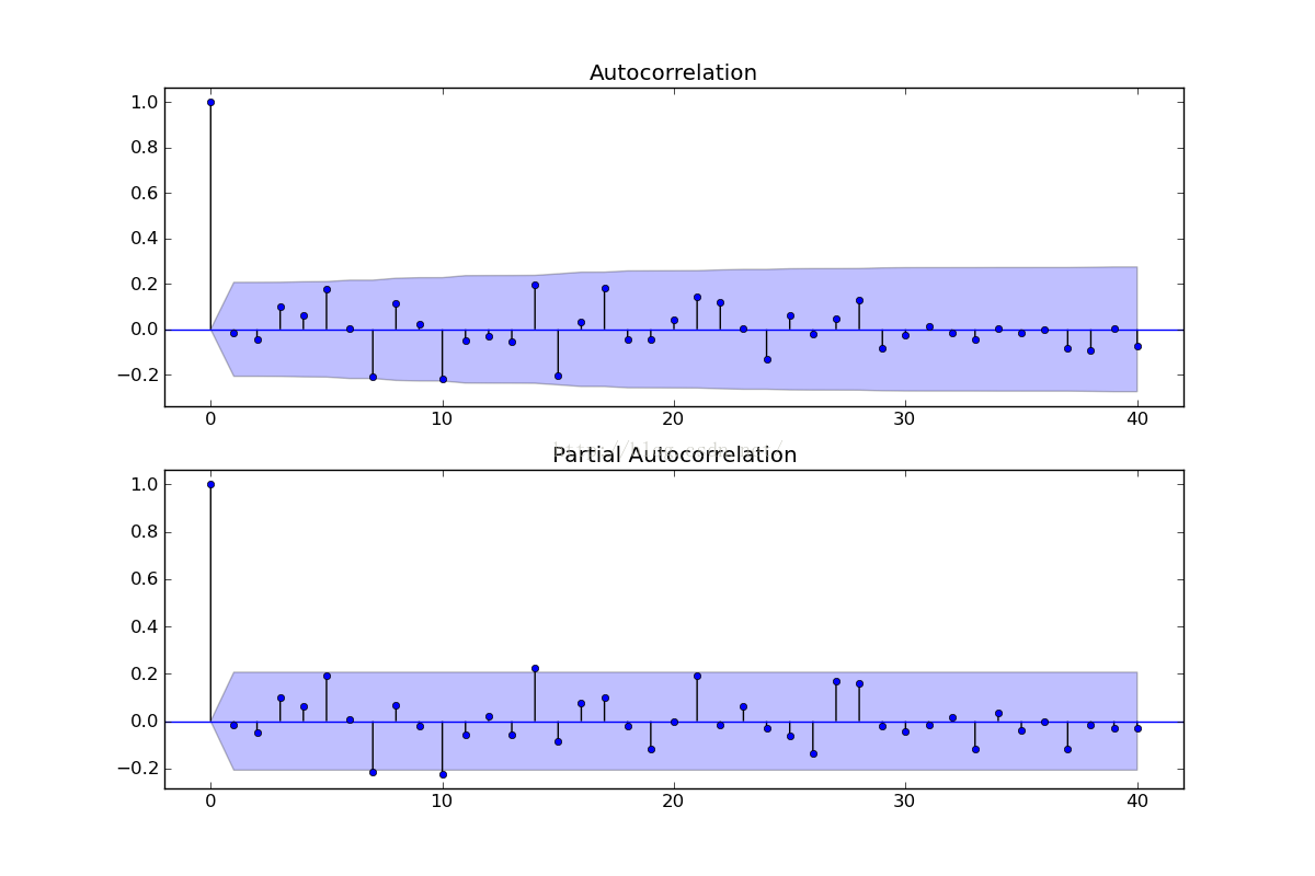
3.3 接下来检验下残差序列:
resid = arma_mod80.resid //原文把这个变量赋值语句漏了,所以老是出错
fig = plt.figure(figsize=(12,8))
ax1 = fig.add_subplot(211)
fig = sm.graphics.tsa.plot_acf(resid.values.squeeze(), lags=40, ax=ax1)
ax2 = fig.add_subplot(212)
fig = sm.graphics.tsa.plot_pacf(resid, lags=40, ax=ax2)
plt.show()
残差的ACF和PACF图,可以看到序列残差基本为白噪声
进一步进行D-W检验,德宾-沃森(Durbin-Watson)检验。德宾-沃森检验,简称D-W检验,是目前检验自相关性最常用的方法,但它只使用于检验一阶自相关性。因为自相关系数ρ的值介于-1和1之间,所以 0≤DW≤4。并且DW=O=>ρ=1 即存在正自相关性
DW=4<=>ρ=-1 即存在负自相关性
DW=2<=>ρ=0 即不存在(一阶)自相关性
因此,当DW值显著的接近于O或4时,则存在自相关性,而接近于2时,则不存在(一阶)自相关性。这样只要知道DW统计量的概率分布,在给定的显著水平下,根据临界值的位置就可以对原假设H0进行检验。
print(sm.stats.durbin_watson(arma_mod80.resid.values))
结果=2.02332930932,所以残差序列不存在自相关性。
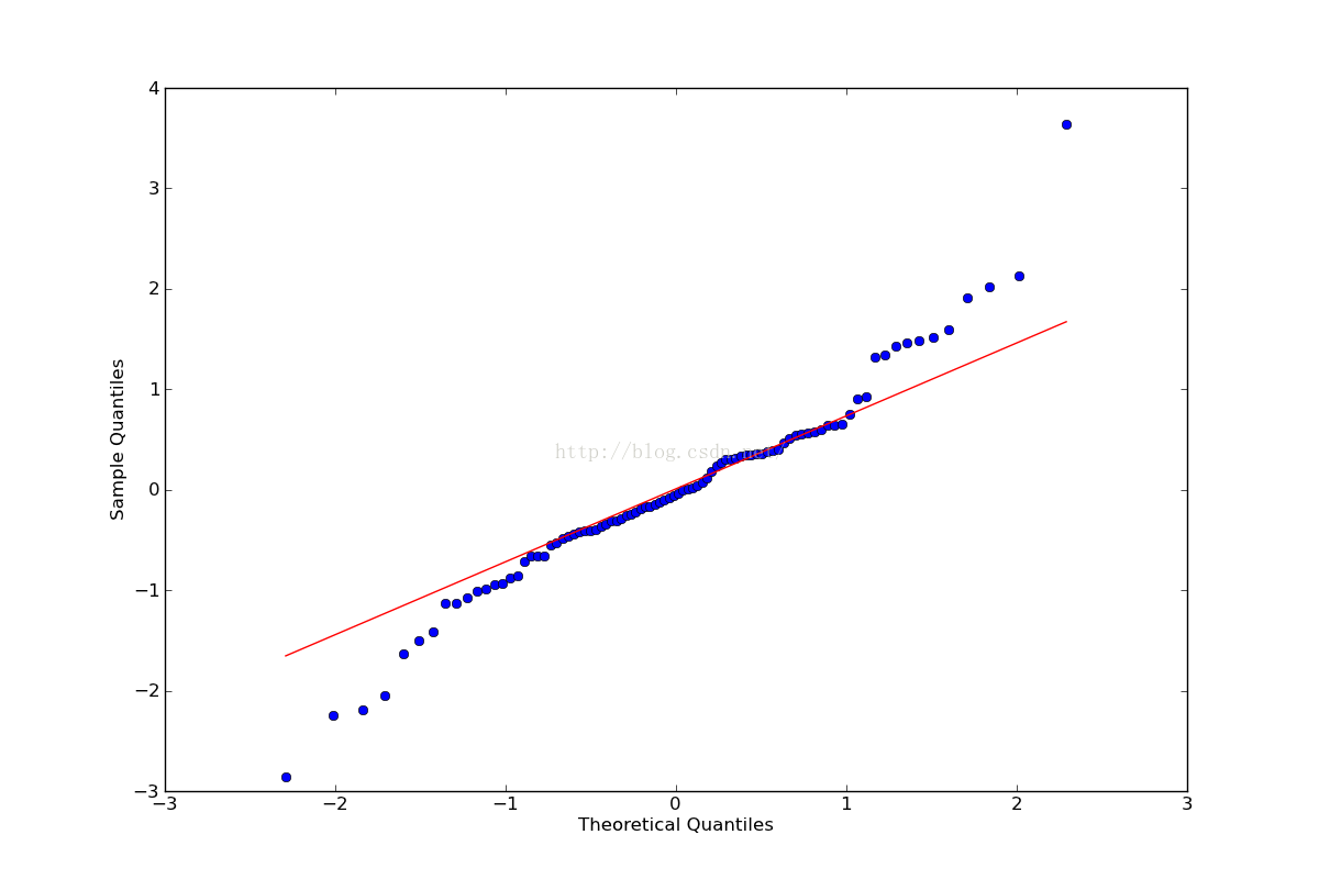
3.4 观察是否符合正态分布
这里使用QQ图,它用于直观验证一组数据是否来自某个分布,或者验证某两组数据是否来自同一(族)分布。
print(stats.normaltest(resid))
fig = plt.figure(figsize=(12,8))
ax = fig.add_subplot(111)
fig = qqplot(resid, line='q', ax=ax, fit=True)
#plt.show()
结果表明基本符合正态分布
3.5 残差序列Ljung-Box检验,也叫Q检验
r,q,p = sm.tsa.acf(resid.values.squeeze(), qstat=True)
data = np.c_[range(1,41), r[1:], q, p]
table = pd.DataFrame(data, columns=['lag', "AC", "Q", "Prob(>Q)"])
print(table.set_index('lag'))
结果:
AC Q Prob(>Q)
lag
1.0 -0.014746 0.020229 0.886899
2.0 -0.045590 0.215795 0.897720
3.0 0.101588 1.197979 0.753489
4.0 0.063346 1.584316 0.811608
5.0 0.176146 4.606765 0.465727
6.0 0.004994 4.609224 0.594816
7.0 -0.209083 8.970252 0.254799
8.0 0.115683 10.321552 0.243178
9.0 0.020911 10.366252 0.321657
10.0 -0.220114 15.380865 0.118781
11.0 -0.050668 15.649938 0.154632
12.0 -0.031545 15.755573 0.202690
13.0 -0.055370 16.085244 0.244557
14.0 0.195340 20.242428 0.122682
15.0 -0.204417 24.855630 0.051916
16.0 0.034558 24.989255 0.070015
17.0 0.181463 28.724206 0.037155
18.0 -0.043332 28.940139 0.049116
19.0 -0.045327 29.179739 0.063210
20.0 0.044198 29.410802 0.079980
21.0 0.141917 31.827664 0.060944
22.0 0.118171 33.528034 0.054822
23.0 0.004488 33.530524 0.072258
24.0 -0.133612 35.770166 0.057769
25.0 0.061816 36.256927 0.067791
26.0 -0.021829 36.318576 0.085964
27.0 0.047270 36.612251 0.102536
28.0 0.131287 38.914114 0.082314
29.0 -0.080915 39.802824 0.087213
30.0 -0.026180 39.897408 0.106867
31.0 0.011463 39.915849 0.130949
32.0 -0.015224 39.948936 0.157836
33.0 -0.042675 40.213480 0.181101
34.0 0.006060 40.218910 0.214085
35.0 -0.015980 40.257355 0.248807
36.0 0.000413 40.257381 0.287349
37.0 -0.083807 41.354656 0.286211
38.0 -0.091967 42.701428 0.276142
39.0 0.002435 42.702391 0.315032
40.0 -0.071601 43.551379 0.322770
prob值均大于0.05,所以残差序列不存在自相关性
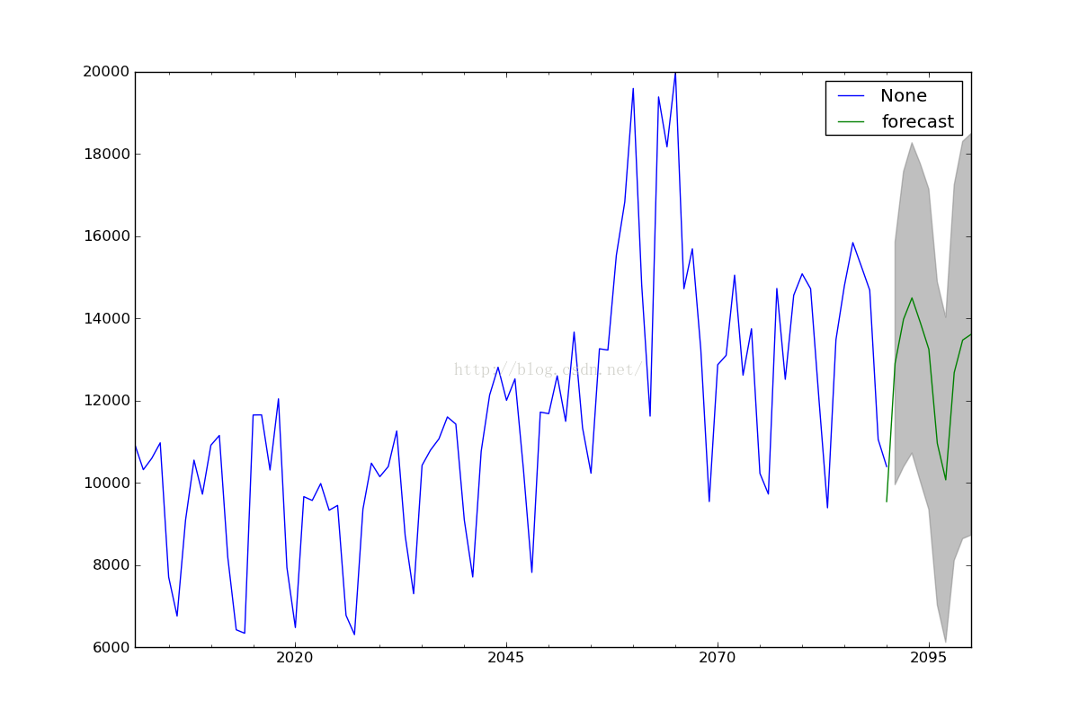
4. 预测
predict_dta = arma_mod80.predict('2090', '2100', dynamic=True)
print(predict_dta)
fig, ax = plt.subplots(figsize=(12, 8))
ax = dta.ix['2000':].plot(ax=ax)
fig = arma_mod80.plot_predict('2090', '2100', dynamic=True, ax=ax, plot_insample=False)
plt.show()
结果:
2090-12-31 9541.934170
2091-12-31 12906.497016
2092-12-31 13979.448587
2093-12-31 14499.448647
2094-12-31 13892.217206
2095-12-31 13247.336277
2096-12-31 10958.837240
2097-12-31 10070.285452
2098-12-31 12680.448582
2099-12-31 13472.910370
2100-12-31 13611.974609
结尾
1.模型的好坏暂时还没查到如何检验,比如APE,MAPE等等
2.系统还有2个报错,虽然不影响结果,原因待查
D:\Python27\lib\site-packages\statsmodels\tsa\arima_model.py:1724: FutureWarning: TimeSeries is deprecated. Please use Series
forecast = TimeSeries(forecast, index=self.data.predict_dates)
D:\Python27\lib\site-packages\matplotlib\collections.py:446: FutureWarning: elementwise comparison failed; returning scalar instead, but in the future will perform elementwise comparison
if self._edgecolors == 'face':
3. 另外还参考了官方的example,http://statsmodels.sourceforge.net/devel/examples/notebooks/generated/tsa_arma_0.html
总体代码:
from __future__ import print_function
import pandas as pd
import numpy as np
from scipy import  stats
import matplotlib.pyplot as plt
import statsmodels.api as sm
from statsmodels.graphics.api import qqplot
# 1数据准备
dta=[10930,10318,10595,10972,7706,6756,9092,10551,9722,10913,11151,8186,6422,
6337,11649,11652,10310,12043,7937,6476,9662,9570,9981,9331,9449,6773,6304,9355,
10477,10148,10395,11261,8713,7299,10424,10795,11069,11602,11427,9095,7707,10767,
12136,12812,12006,12528,10329,7818,11719,11683,12603,11495,13670,11337,10232,
13261,13230,15535,16837,19598,14823,11622,19391,18177,19994,14723,15694,13248,
9543,12872,13101,15053,12619,13749,10228,9725,14729,12518,14564,15085,14722,
11999,9390,13481,14795,15845,15271,14686,11054,10395]
dta=np.array(dta,dtype=np.float)
dta=pd.Series(dta)
#dta=pd.tseries(dta)
dta.index = pd.Index(sm.tsa.datetools.dates_from_range('2001','2090')) #应该是2090,不是2100
dta.plot(figsize=(12,8))

plt.show()
# 2时间序列的差分d
fig = plt.figure(figsize=(12,8))
ax1= fig.add_subplot(111)
diff1 = dta.diff(1)
diff1.plot(ax=ax1)
## 3合适的p,q
# 3.1检查平稳时间序列的自相关图和偏自相关图
diff1= dta.diff(1)#我们已经知道要使用一阶差分的时间序列,之前判断差分的程序可以注释掉
fig = plt.figure(figsize=(12,8))
ax1=fig.add_subplot(211)
fig = sm.graphics.tsa.plot_acf(dta,lags=40,ax=ax1)
ax2 = fig.add_subplot(212)
fig = sm.graphics.tsa.plot_pacf(dta,lags=40,ax=ax2)
# 3.2模型选择
arma_mod70 = sm.tsa.ARMA(dta,(7,0)).fit()
print(arma_mod70.aic,arma_mod70.bic,arma_mod70.hqic)
arma_mod30 = sm.tsa.ARMA(dta,(0,1)).fit()
print(arma_mod30.aic,arma_mod30.bic,arma_mod30.hqic)
arma_mod71 = sm.tsa.ARMA(dta,(7,1)).fit()
print(arma_mod71.aic,arma_mod71.bic,arma_mod71.hqic)
arma_mod80 = sm.tsa.ARMA(dta,(8,0)).fit()
print(arma_mod80.aic,arma_mod80.bic,arma_mod80.hqic)
# 3.3 检验残差序列
resid = arma_mod80.resid
fig = plt.figure(figsize=(12,8))
ax1 = fig.add_subplot(211)
fig = sm.graphics.tsa.plot_acf(resid.values.squeeze(), lags=40, ax=ax1)
ax2 = fig.add_subplot(212)
fig = sm.graphics.tsa.plot_pacf(resid, lags=40, ax=ax2)
plt.show()
print(sm.stats.durbin_watson(arma_mod80.resid.values))
# 3.4 观察是否正太分布
print(stats.normaltest(resid))
fig = plt.figure(figsize=(12,8))
ax = fig.add_subplot(111)
fig = qqplot(resid, line='q', ax=ax, fit=True)
#plt.show()
# 3.5残差序列检验
r,q,p = sm.tsa.acf(resid.values.squeeze(), qstat=True)
data = np.c_[range(1,41), r[1:], q, p]
table = pd.DataFrame(data, columns=['lag', "AC", "Q", "Prob(>Q)"])
print(table.set_index('lag'))

predict_dta = arma_mod80.predict('2090', '2100', dynamic=True)
print(predict_dta)

# 3.6预测
fig, ax = plt.subplots(figsize=(12, 8))
ax = dta.ix['2000':].plot(ax=ax)
fig = arma_mod80.plot_predict('2090', '2100', dynamic=True, ax=ax, plot_insample=False)
plt.show()