1.背景
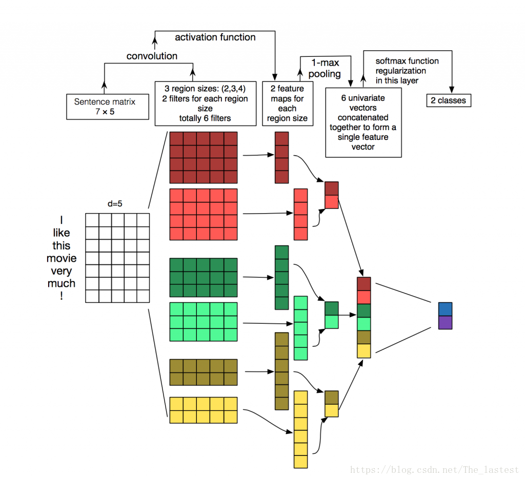
如图,最左边部分是一个句子构成的2维矩阵(可以理解为通道为1的图片),其形状为shape=[7,5,1]。图中:
第一步:先用3个卷积核进行了卷积操作,即卷积核的形状分别为shape1=[4,5,1,2],shape2=[3,4,1,2],shape3=[2,4,1,2];卷积后的形状分别为[4,1,2],[5,1,2],[6,1,2];
第二步:采用max pool进行池化操作,池化后的形状均为[1,1,2];
第三步:将这6个部分叠加起来,然后进行全连接处理;
看着这个图理解一般都没有问题,唯一的问题可能就是出现在编码的时候。而且只要这个问题清楚了,对应这一类简单的拼接就应该会了。
2.理论计算
假设现在有两张图片(形状为[6,3,1]),分别用一个向量保存着(这也是实际数据中最常见的形式),所以首先要做的就是reshape。
a = tf.constant([[1,2,3,4,5,6,7,8,9,10,11,12,17,18,19,20,21,22],
                 [4,5,6,4,3,5,8,9,0,6,4,3,1,3,5,7,4,3]],shape=[2,18],dtype=tf.float32,name='a')
理论上的形状:
# 1   2   3       4   5   6
# 4   5   6       4   3   5
# 7   8   9       8   9   0
# 10  11  12      6   4   3
# 17  18  19      1   3   5
# 20  21  22      7   4   3
2.1 convolution
为了方便后面验证,我们令所有卷积核和偏置的参数均为1,3种尺寸分别为[2,3,1,2],[3,3,1,2],[4,3,1,2]则:
对于第一张图采用这3种形状的核,卷积后处理后的结果分别为:
        22  22          46  46          79  79
        40  40          73  73          127 127
        58  58          112 112         175 175
        88  88          151 151
        118 118
#shape  [5,1,1,2]       [4,1,1,2]       [3,1,1,2]
对于第二张图采用这3种形状的核,卷积后处理后的结果分别为:
        28  28          45  45          58  58
        30  30          43  43          52  52
        31  31          40  40          54  54
        23  23          37  37
        24  24
#shape  [5,1,1,2]       [4,1,1,2]       [3,1,1,2]
2.2 max pool
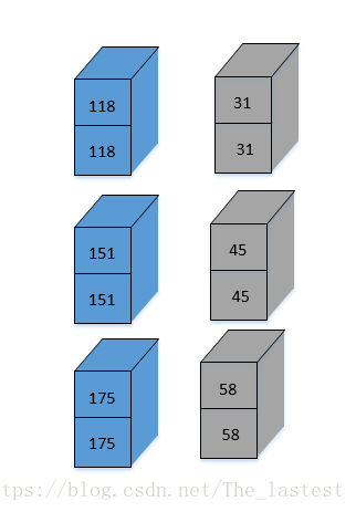
对于第一张图采用max pool 处理后的结果为:
        118 118         151 151        175 175
#shape  [1,1,1,2]       [1,1,1,2]       [1,1,1,2]
对于第二张图采用max pool 处理后的结果为:
31 31 45 45 58 58
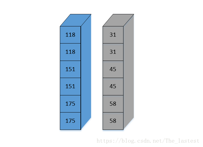
#shape [1,1,1,2] [1,1,1,2] [1,1,1,2] 2.3 concat and reshape
[[ 118.  118.  151.  151.  175.  175.]
 [  31.   31.   45.   45.   58.   58.]]
3.tensorflow实现
3.1 reshape
a = tf.constant([[1,2,3,4,5,6,7,8,9,10,11,12,17,18,19,20,21,22],
                 [4,5,6,4,3,5,8,9,0,6,4,3,1,3,5,7,4,3]],shape=[2,18],dtype=tf.float32,name='a')
reshaped_a = tf.reshape(a,shape=[2,6,3,1])这里每张图为18维,shape=[2,6,3,1]指的是2张图,每张图的大小是[6,3],通道为1.
输出后是这种形式:
[[[[  1.]
   [  2.]
   [  3.]]

  [[  4.]
   [  5.]
   [  6.]]

  [[  7.]
   [  8.]
   [  9.]]

  [[ 10.]
   [ 11.]
   [ 12.]]

  [[ 17.]
   [ 18.]
   [ 19.]]

  [[ 20.]
   [ 21.]
   [ 22.]]]


 [[[  4.]
   [  5.]
   [  6.]]

  [[  4.]
   [  3.]
   [  5.]]

  [[  8.]
   [  9.]
   [  0.]]

  [[  6.]
   [  4.]
   [  3.]]

  [[  1.]
   [  3.]
   [  5.]]

  [[  7.]
   [  4.]
   [  3.]]]]

Tensor("Reshape:0", shape=(2, 6, 3, 1), dtype=float32)
这种形式看起来确实不怎么好理解,不过可以通过程序的结果输出来验证其正确性。
3.2 convolution and max pool
a = tf.constant([[1,2,3,4,5,6,7,8,9,10,11,12,17,18,19,20,21,22],
                 [4,5,6,4,3,5,8,9,0,6,4,3,1,3,5,7,4,3]],shape=[2,18],dtype=tf.float32,name='a')
reshaped_a = tf.reshape(a,shape=[2,6,3,1])

filter_size = [2,3,4]
c = []
pool = []

for filters in filter_size:
    with tf.name_scope("conv-maxpool-%s" % filters):
        filter_shape = [filters,3,1,2]
        W = tf.constant(1.0,shape=filter_shape)
        b = tf.constant(1.0,shape=[2])
        conv = tf.nn.conv2d(input = reshaped_a,filter=W,strides=[1,1,1,1],padding='VALID')
        convs=tf.nn.bias_add(conv,b)
        c.append(convs)
        pooled = tf.nn.max_pool(value=convs,ksize=[1,6-filters+1,1,1],strides=[1,1,1,1],padding='VALID')
        pool.append(pooled)
h_pool = tf.concat(values=pool,name='last_pool_layer',axis=3)
h_pool_flat = tf.reshape(tensor=h_pool,shape=[-1,6])

with tf.Session() as sess:
    print(sess.run(c))
    print(sess.run(pool))
为了方便观察,我们用了两个List来分别保存卷积和池化后的结果。
#卷积后的结果
#-------------------------------------part 1
[array([[[[  22.,   22.]],

        [[  40.,   40.]],

        [[  58.,   58.]],

        [[  88.,   88.]],

        [[ 118.,  118.]]],


       [[[  28.,   28.]],

        [[  30.,   30.]],

        [[  31.,   31.]],

        [[  23.,   23.]],

        [[  24.,   24.]]]], dtype=float32),
#-------------------------------------part 2
array([[[[  46.,   46.]],

        [[  73.,   73.]],

        [[ 112.,  112.]],

        [[ 151.,  151.]]],


       [[[  45.,   45.]],

        [[  43.,   43.]],

        [[  40.,   40.]],

        [[  37.,   37.]]]], dtype=float32),
#-------------------------------------part 3
array([[[[  79.,   79.]],

        [[ 127.,  127.]],

        [[ 175.,  175.]]],


       [[[  58.,   58.]],

        [[  52.,   52.]],

        [[  54.,   54.]]]], dtype=float32)]
可以发现,卷积后三个部分的结果与上面的理论结果一样
#池化后的结果
[array([[[[ 118.,  118.]]],[[[  31.,   31.]]]], dtype=float32), array([[[[ 151.,  151.]]],[[[  45.,   45.]]]], dtype=float32), array([[[[ 175.,  175.]]],[[[  58.,   58.]]]], dtype=float32)]
对应如下:
h_pool = tf.concat(values=pool,name='last_pool_layer',axis=3)
#[[[[ 118.  118.  151.  151.  175.  175.]]]
# [[[  31.   31.   45.   45.   58.   58.]]]]
如下:
h_pool_flat = tf.reshape(tensor=h_pool,shape=[-1,6])
#[[ 118.  118.  151.  151.  175.  175.]
# [  31.   31.   45.   45.   58.   58.]]