0. 引言
VGGNet,由Simonyan和Zisserman在2014年提出,论文名字是《Very Deep Learning Convolutional Neural Networks for Large-Scale Image Recognition》。他们做出的贡献主要是提出了一个只用(3x3)的卷积filters,并且层数为16-19层的神经网络。使用这个网络,在ImageNet分类挑战中,可以获得较高的分类精度。(笔者到现在的学习过程中,发现最神经网络的结构越简单,训练速度较快,但是识别精度不高。因此是需要使用前人已经验证过了有较高识别精度的网络结构。)
本文为了先让大家一起体会一下VGGNet的深度,把VGGNet的复杂度适当的降低到只有两层结构,并将其命名为MiniVGGNet。以尊重原创。
1. MiniVGGNet的网络结构
第一层:INPUT =>
第二层:CONV => ACT => BN => CONV => ACT =>BN => POOL => DROPOUT =>
第三层:CONV => ACT => BN => CONV => ACT =>BN => POOL => DROPOUT =>
第四层:FC => ACT => BN => DROPOUT =>
第五层:FC => SOFTMAX
| Layer Type | Output Size | Filter Size / Stride |
| INPUT IMAGE | 32 x 32 x 3 | |
| CONV | 32 x 32 x 32 | 3 x 3, K = 32 |
| ACT | 32 x 32 x 32 | |
| BN | 32 x 32 x 32 | |
| CONV | 32 x 32 x 32 | 3 x 3, K = 32 |
| ACT | 32 x 32 x 32 | |
| BN | 32 x 32 x 32 | |
| POOL | 16 x 16 x 32 | 2 x 2 |
| DROPOUT | 16 x 16 x 32 | |
| CONV | 16 x 16 x 64 | 3 x 3, K = 64 |
| ACT | 16 x 16 x 64 | |
| BN | 16 x 16 x 64 | |
| CONV | 16 x 16 x 64 | 3 x 3, K = 64 |
| ACT | 16 x 16 x 64 | |
| BN | 16 x 16 x 64 | |
| POOL | 8 x 8 x 64 | 2 x 2 |
| DROPOUT | 8 x 8 x 64 | |
| FC | 512 | |
| ACT | 512 | |
| BN | 5212 | |
| DROPOUT | 512 | |
| FC | 10 | |
| SOFTMAX | 10 |
VGGNet会不断重复上述的第2层和第3层,叠加知道总体的层数到达16层到19层之间。这样大大的增加了网络的复杂性。也增加了训练所需的消耗。
2. 代码
2.1 minivggnet.py
# import the necessary packages
from keras.models import Sequential
from keras.layers.normalization import BatchNormalization
from keras.layers.convolutional import Conv2D
from keras.layers.convolutional import MaxPooling2D
from keras.layers.core import Activation
from keras.layers.core import Flatten
from keras.layers.core import Dropout
from keras.layers.core import Dense
from keras import backend as K

class MiniVGGNet:
	@staticmethod
	def build(width, height, depth, classes):
		# initialize the model along with the input shape to be
		# "channels last" and the channels dimension itself
		model = Sequential()
		inputShape = (height, width, depth)
		chanDim = -1

		# if we are using "channels first", update the input shape
		# and channels dimension
		if K.image_data_format() == "channels_first":
			inputShape = (depth, height, width)
			chanDim = 1

		# first CONV => RELU => CONV => RELU => POOL layer set
		model.add(Conv2D(32, (3, 3), padding="same",
			input_shape=inputShape))
		model.add(Activation("relu"))
		model.add(BatchNormalization(axis=chanDim))
		model.add(Conv2D(32, (3, 3), padding="same"))
		model.add(Activation("relu"))
		model.add(BatchNormalization(axis=chanDim))
		model.add(MaxPooling2D(pool_size=(2, 2)))
		model.add(Dropout(0.25))

		# second CONV => RELU => CONV => RELU => POOL layer set
		model.add(Conv2D(64, (3, 3), padding="same"))
		model.add(Activation("relu"))
		model.add(BatchNormalization(axis=chanDim))
		model.add(Conv2D(64, (3, 3), padding="same"))
		model.add(Activation("relu"))
		model.add(BatchNormalization(axis=chanDim))
		model.add(MaxPooling2D(pool_size=(2, 2)))
		model.add(Dropout(0.25))

		# first (and only) set of FC => RELU layers
		model.add(Flatten())
		model.add(Dense(512))
		model.add(Activation("relu"))
		model.add(BatchNormalization())
		model.add(Dropout(0.5))

		# softmax classifier
		model.add(Dense(classes))
		model.add(Activation("softmax"))

		# return the constructed network architecture
		return model
2.2 minivggnet_cifar10.py
本代码会调用keras.datasets的cifar10,当运行cifar10.load_data(),系统会自动下载cifar10数据集。Windows下面会下载到c:\Users\<用户名>\.keras\datasets。
Ubuntu下会自动下载到~/.keras/datasets。我因为已经在Ubuntu18电脑内下载过一次,于是把该tar.gz压缩文件复制到datasets文件夹内即可。注意的是,服务器上,压缩包名字cifar-10-python.tar.gz。Keras会把文件改名为cifar-10-batches-py.tar.gz。因此如果自行从服务器下载的话,需要把名字改为keras所识别的名字。
# set the matplotlib backend so figures can be saved in the background
import matplotlib
matplotlib.use("Agg")

# import the necessary packages
from sklearn.preprocessing import LabelBinarizer
from sklearn.metrics import classification_report
from pyimagesearch.nn.conv import MiniVGGNet
from keras.optimizers import SGD
from keras.datasets import cifar10
import matplotlib.pyplot as plt
import numpy as np
import argparse

# construct the argument parse and parse the arguments
ap = argparse.ArgumentParser()
ap.add_argument("-o", "--output", required=True,
	help="path to the output loss/accuracy plot")
args = vars(ap.parse_args())

# load the training and testing data, then scale it into the
# range [0, 1]
print("[INFO] loading CIFAR-10 data...")
((trainX, trainY), (testX, testY)) = cifar10.load_data()
trainX = trainX.astype("float") / 255.0
testX = testX.astype("float") / 255.0

# convert the labels from integers to vectors
lb = LabelBinarizer()
trainY = lb.fit_transform(trainY)
testY = lb.transform(testY)

# initialize the label names for the CIFAR-10 dataset
labelNames = ["airplane", "automobile", "bird", "cat", "deer",
	"dog", "frog", "horse", "ship", "truck"]

# initialize the optimizer and model
print("[INFO] compiling model...")
opt = SGD(lr=0.01, decay=0.01 / 40, momentum=0.9, nesterov=True)
model = MiniVGGNet.build(width=32, height=32, depth=3, classes=10)
model.compile(loss="categorical_crossentropy", optimizer=opt,
	metrics=["accuracy"])

# train the network
print("[INFO] training network...")
H = model.fit(trainX, trainY, validation_data=(testX, testY),
	batch_size=64, epochs=40, verbose=1)

# evaluate the network
print("[INFO] evaluating network...")
predictions = model.predict(testX, batch_size=64)
print(classification_report(testY.argmax(axis=1),
	predictions.argmax(axis=1), target_names=labelNames))

# plot the training loss and accuracy
plt.style.use("ggplot")
plt.figure()
plt.plot(np.arange(0, 40), H.history["loss"], label="train_loss")
plt.plot(np.arange(0, 40), H.history["val_loss"], label="val_loss")
plt.plot(np.arange(0, 40), H.history["acc"], label="train_acc")
plt.plot(np.arange(0, 40), H.history["val_acc"], label="val_acc")
plt.title("Training Loss and Accuracy on CIFAR-10")
plt.xlabel("Epoch #")
plt.ylabel("Loss/Accuracy")
plt.legend()
plt.savefig(args["output"])
3. 运行结果
执行指令
python minivggnet_cifar10.py --output output/cifar10_minivggnet_with_no_bn.png经历了漫长的等待。
我的电脑是i3-6100的台式机。内存为8G。CPU的Tensorflow。一次迭代需要356s。中午差几分12:00开始跑的,要到15:35左右才完成了40次迭代运算。
Epoch 40/40
   64/50000 [..............................] - ETA: 5:39 - loss: 0.2286 - acc: 0
   128/50000 [..............................] - ETA: 5:39 - loss: 0.2074 - acc: 0
   192/50000 [..............................] - ETA: 5:38 - loss: 0.1949 - acc: 0
   256/50000 [..............................] - ETA: 5:38 - loss: 0.2003 - acc: 0
   15552/50000 [========>.....................] - ETA: 3:54 - loss: 0.2430 - acc: 0
   48256/50000 [===========================>..] - ETA: 11s - loss: 0.2494 - acc: 0
   49920/50000 [============================>.] - ETA: 0s - loss: 0.2487 - acc: 0.9
   49984/50000 [============================>.] - ETA: 0s - loss: 0.2488 - acc: 0.9
   50000/50000 [==============================] - 356s 7ms/step - loss: 0.2488 - acc: 0.9100 - val_loss: 0.5595 - val_acc: 0.8224

[INFO] evaluating network...
             precision    recall  f1-score   support

   airplane       0.83      0.82      0.83      1000
 automobile       0.89      0.93      0.91      1000
       bird       0.74      0.76      0.75      1000
        cat       0.70      0.64      0.67      1000
       deer       0.81      0.78      0.80      1000
        dog       0.75      0.75      0.75      1000
       frog       0.82      0.90      0.86      1000
      horse       0.91      0.84      0.87      1000
       ship       0.88      0.92      0.90      1000
      truck       0.88      0.88      0.88      1000

avg / total       0.82      0.82      0.82     10000
另外迭代结果可以查看 output文件夹中的cifar10-minivggnet-with-bn.png
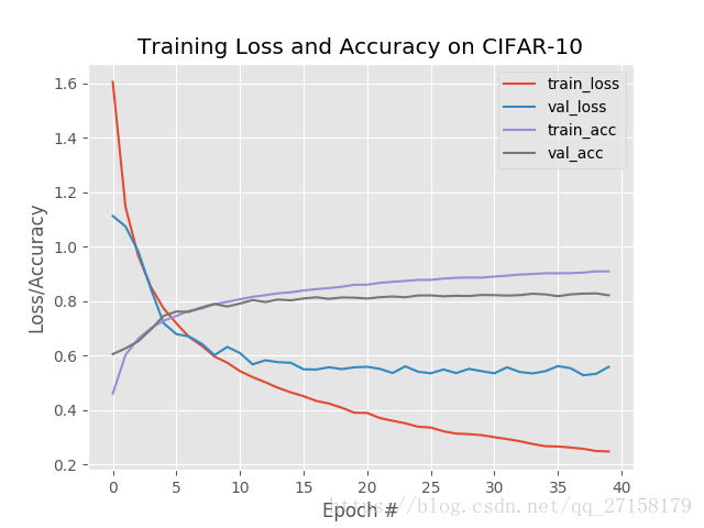
从结果来看,MiniVGGNet在Cifar-10数据集的成绩是:平均识别精度达到了82%。跟我之前运行的ShallowNet比起来,高了20个百分点。精度有了很大改进。
代码全部来自:《Deep.Learning.for.Computer.Vision.with.Python.Starter.Bundle.2017.9.pdf》。推荐一看。