vs2017 VGG19处理cifar-10数据集--更进一步的学习tensorflow相关知识

版权声明：本文为博主原创文章，未经博主允许不得转载。 https://blog.csdn.net/qq_36556893/article/details/85046067

这是针对于博客vs2017安装和使用教程（详细）的VGG19-CIFAR10项目新建示例

---

目录

一、代码(附有重要的注释)

二、项目结构

三、VGG简介

四、程序执行关键部分解析

五、训练过程和结果

六、参考博客和文献

---

一、代码(附有重要的注释)

1.博主提供的代码包含了很多重要的注释，都是博主精心查阅资料和debug的结果，对于新手了解tensorflow使用以及深度学习框架十分有用。

2.代码如下：

vgg19.py

import tensorflow as tf
import numpy as np
import time
import os
import sys
import pickle
import random


class_num = 10
image_size = 32
img_channels = 3
iterations = 200
batch_size = 250
total_epoch = 164
weight_decay = 0.0003
dropout_rate = 0.5
momentum_rate = 0.9
log_save_path = './vgg_logs'
model_save_path = './model/'


def download_data():
    dirname = 'cifar-10-batches-py'
    origin = 'http://www.cs.toronto.edu/~kriz/cifar-10-python.tar.gz'
    fname = './CAFIR-10_data/cifar-10-python.tar.gz'
    fpath = './' + dirname

    download = False
    if os.path.exists(fpath) or os.path.isfile(fname):
        download = False
        print("DataSet already exist!")
    else:
        download = True
    if download:
        print('Downloading data from', origin)
        import urllib.request
        import tarfile

        def reporthook(count, block_size, total_size):
            global start_time
            if count == 0:
                start_time = time.time()
                return
            duration = time.time() - start_time
            progress_size = int(count * block_size)
            speed = int(progress_size / (1024 * duration))
            percent = min(int(count*block_size*100/total_size),100)
            sys.stdout.write("\r...%d%%, %d MB, %d KB/s, %d seconds passed" %
                            (percent, progress_size / (1024 * 1024), speed, duration))
            sys.stdout.flush()

        urllib.request.urlretrieve(origin, fname, reporthook)
        print('Download finished. Start extract!', origin)
        if fname.endswith("tar.gz"):
            tar = tarfile.open(fname, "r:gz")
            tar.extractall()
            tar.close()
        elif fname.endswith("tar"):
            tar = tarfile.open(fname, "r:")
            tar.extractall()
            tar.close()


def unpickle(file):
    with open(file, 'rb') as fo:
        dict = pickle.load(fo, encoding='bytes')
    return dict


def load_data_one(file):
    batch = unpickle(file)#./cifar-10-batches-py/data_batch_1 ./cifar-10-batches-py/test_batch'
    data = batch[b'data']#数据
    labels = batch[b'labels']#标签
    print("Loading %s : %d." % (file, len(data)))
    return data, labels


def load_data(files, data_dir, label_count):
    global image_size, img_channels
    data, labels = load_data_one(data_dir + '/' + files[0])#./cifar-10-batches-py/data_batch_1 [0:10000]
    for f in files[1:]:#test_batch时不经历该循环
        data_n, labels_n = load_data_one(data_dir + '/' + f)#从./cifar-10-batches-py/data_batch_2
        data = np.append(data, data_n, axis=0)#在行末尾追加，第一次循环变为[0:20000]
        labels = np.append(labels, labels_n, axis=0)#最终[0:50000]
    labels = np.array([[float(i == label) for i in range(label_count)] for label in labels])#labels重组，原数组第i个数字为k则第i行第k个位置位1，其它位置为0
    #print(labels)
    data = data.reshape([-1, img_channels, image_size, image_size])#-1缺省，函数自己计算，这里为train:50000 test:10000
    data = data.transpose([0, 2, 3, 1])#train:[50000,3,32,32]变成[50000,32,32,3] test:[10000,3,32,32]变成[10000,32,32,3]
    return data, labels


def prepare_data():
    print("======Loading data======")
    download_data()
    data_dir = './cifar-10-batches-py'
    image_dim = image_size * image_size * img_channels #32x32x3
    meta = unpickle(data_dir + '/batches.meta')

    label_names = meta[b'label_names']#[b'airplane', b'automobile', b'bird', b'cat', b'deer', b'dog', b'frog', b'horse', b'ship', b'truck']
    label_count = len(label_names)#10
    train_files = ['data_batch_%d' % d for d in range(1, 6)]#['data_batch_1', 'data_batch_2', 'data_batch_3', 'data_batch_4', 'data_batch_5']
    train_data, train_labels = load_data(train_files, data_dir, label_count)#train_data[50000,32,32,3],train_labels[0,50000]
    test_data, test_labels = load_data(['test_batch'], data_dir, label_count)

    print("Train data:", np.shape(train_data), np.shape(train_labels))#Train data: (50000, 32, 32, 3) (50000, 10)
    print("Test data :", np.shape(test_data), np.shape(test_labels))#Test data : (10000, 32, 32, 3) (10000, 10)
    print("======Load finished======")#训练和测试数据读取完成

    print("======Shuffling data======")
    indices = np.random.permutation(len(train_data))#返回一个0-50000的随机排列
    train_data = train_data[indices]#train重新排列
    train_labels = train_labels[indices]#test重新排列
    print("======Prepare Finished======")

    return train_data, train_labels, test_data, test_labels


def bias_variable(shape):
    initial = tf.constant(0.1, shape=shape, dtype=tf.float32)# <tf.Tensor 'Const:0' shape=(64,) dtype=float32>
    return tf.Variable(initial)


def conv2d(x, W):
    #x:指需要做卷积的输入图像，它要求是一个Tensor，
    #具有[batch, in_height, in_width, in_channels]这样的shape，
    #具体含义是[训练时一个batch的图片数量, 图片高度, 图片宽度, 图像通道数]，
    #注意这是一个4维的Tensor，要求类型为float32和float64其中之一
    #W:相当于CNN中的卷积核，它要求是一个Tensor，
    #具有[filter_height, filter_width, in_channels, out_channels]这样的shape，
    #具体含义是[卷积核的高度，卷积核的宽度，图像通道数，卷积核个数]，
    #要求类型与参数input相同，
    #有一个地方需要注意，第三维in_channels，就是参数input的第四维
    #strides:卷积时在图像每一维的步长，这是一个一维的向量，长度4
    #padding:string类型的量，只能是"SAME","VALID"其中之一，这个值决定了不同的卷积方式
    #padding = 'SAME':补0,受到strides大小影响
    return tf.nn.conv2d(x, W, strides=[1, 1, 1, 1], padding='SAME')

#
def max_pool(input, k_size=1, stride=1, name=None):
    #input:需要池化的输入，一般池化层接在卷积层后面，所以输入通常是feature map，
    #依然是[batch, height, width, channels]这样的shape
    #ksize：池化窗口的大小，取一个四维向量，一般是[1, height, width, 1]，
    #因为我们不想在batch和channels上做池化，所以这两个维度设为了1
    #strides：和卷积类似，窗口在每一个维度上滑动的步长，一般也是[1, stride,stride, 1]
    #padding：和卷积类似，可以取'VALID' 或者'SAME'
    #返回一个Tensor，类型不变，shape仍然是[batch, height, width, channels]这种形式
    return tf.nn.max_pool(input, ksize=[1, k_size, k_size, 1], strides=[1, stride, stride, 1],
                          padding='SAME', name=name)

#公式如下：
#y=γ(x-μ)/σ+β
#其中:
#x是输入，
#y是输出，
#μ是均值，
#σ是方差，
#γ和β是缩放（scale）、偏移（offset）系数。
#一般来讲，这些参数都是基于channel来做的，比如输入x是一个16*32*32*128(NWHC格式)的feature map，
#那么上述参数都是128维的向量。其中γ和β是可有可无的，
#有的话，就是一个可以学习的参数（参与前向后向），
#没有的话，就简化成y=(x-μ)/σ。
#而μ和σ，在训练的时候，使用的是batch内的统计值，
#测试/预测的时候，采用的是训练时计算出的滑动平均值。
def batch_norm(input):
    #decay:衰减系数。合适的衰减系数值接近1.0,特别是含多个9的值：0.999,0.99,0.9。
    #如果训练集表现很好而验证/测试集表现得不好，选择小的系数（推荐使用0.9）。
    #如果想要提高稳定性，zero_debias_moving_mean设为True
    #center:如果为True，有beta偏移量；如果为False，无beta偏移量
    #scale:如果为True，则乘以gamma。
    #如果为False，gamma则不使用。
    #当下一层是线性的时（例如nn.relu），由于缩放可以由下一层完成，所以可以禁用该层。
    #epsilon:ε,避免被零除
    #is_training:图层是否处于训练模式。
    #在训练模式下，它将积累转入的统计量moving_mean并 moving_variance使用给定的指数移动平均值 decay。
    #当它不是在训练模式，那么它将使用的数值moving_mean和moving_variance。
    #updates_collections ：Collections来收集计算的更新操作。
    #updates_ops需要使用train_op来执行。
    #如果为None，则会添加控件依赖项以确保更新已计算到位。
    return tf.contrib.layers.batch_norm(input, decay=0.9, center=True, scale=True, epsilon=1e-3,
                                        is_training=train_flag, updates_collections=None)


def _random_crop(batch, crop_shape, padding=None):
    oshape = np.shape(batch[0])#(32, 32, 3)

    if padding:
        oshape = (oshape[0] + 2*padding, oshape[1] + 2*padding)#(40, 40)元组
    new_batch = []
    npad = ((padding, padding), (padding, padding), (0, 0))#((4, 4), (4, 4), (0, 0))
    for i in range(len(batch)):#250
        new_batch.append(batch[i])
        if padding:
            #pad（array，pad_width，mode，**kwars）
            #其中array为要填补的数组（input）
            #pad_width是在各维度的各个方向上想要填补的长度,如（（2，3），（4，5）），
            #如果直接输入一个整数，则说明各个维度和各个方向所填补的长度都一样。
            #mode为填补类型，即怎样去填补，有“constant”，“edge”等模式，
            #如果为constant模式，就得指定填补的值。
            new_batch[i] = np.lib.pad(batch[i], pad_width=npad,
                                      mode='constant', constant_values=0)#边缘填充,[0:32]变成[0,40]
        #temp = oshape[0] - crop_shape[0]
        nh = random.randint(0, oshape[0] - crop_shape[0])#返回[0,8]之间的整数
        nw = random.randint(0, oshape[1] - crop_shape[1])
        new_batch[i] = new_batch[i][nh:nh + crop_shape[0],
                                    nw:nw + crop_shape[1]]#长度为32
    return new_batch


def _random_flip_leftright(batch):
        for i in range(len(batch)):
            if bool(random.getrandbits(1)):#返回一个1位随机的integer
                batch[i] = np.fliplr(batch[i])#左右翻转矩阵
        return batch


def data_preprocessing(x_train,x_test):

    x_train = x_train.astype('float32')#train数据转换为float32
    x_test = x_test.astype('float32')#test数据转换为float32
    #Z-score标准化（0-1标准化）方法，这种方法给予原始数据的均值（mean）和标准差（standard deviation）进行数据的标准化。
    #经过处理的数据符合标准正态分布，即均值为0，标准差为1。
    x_train[:, :, :, 0] = (x_train[:, :, :, 0] - np.mean(x_train[:, :, :, 0])) / np.std(x_train[:, :, :, 0])
    x_train[:, :, :, 1] = (x_train[:, :, :, 1] - np.mean(x_train[:, :, :, 1])) / np.std(x_train[:, :, :, 1])
    x_train[:, :, :, 2] = (x_train[:, :, :, 2] - np.mean(x_train[:, :, :, 2])) / np.std(x_train[:, :, :, 2])

    x_test[:, :, :, 0] = (x_test[:, :, :, 0] - np.mean(x_test[:, :, :, 0])) / np.std(x_test[:, :, :, 0])
    x_test[:, :, :, 1] = (x_test[:, :, :, 1] - np.mean(x_test[:, :, :, 1])) / np.std(x_test[:, :, :, 1])
    x_test[:, :, :, 2] = (x_test[:, :, :, 2] - np.mean(x_test[:, :, :, 2])) / np.std(x_test[:, :, :, 2])

    return x_train, x_test


def data_augmentation(batch):
    batch = _random_flip_leftright(batch)#[0:250]
    batch = _random_crop(batch, [32, 32], 4)#[250,32,32,3]
    return batch


def learning_rate_schedule(epoch_num):
    if epoch_num < 81:
        return 0.1
    elif epoch_num < 121:
        return 0.01
    else:
        return 0.001


def run_testing(sess, ep):
    acc = 0.0
    loss = 0.0
    pre_index = 0
    add = 1000
    for it in range(10):
        batch_x = test_x[pre_index:pre_index+add]
        batch_y = test_y[pre_index:pre_index+add]
        pre_index = pre_index + add
        loss_, acc_  = sess.run([cross_entropy, accuracy],
                                feed_dict={x: batch_x, y_: batch_y, keep_prob: 1.0, train_flag: False})
        loss += loss_ / 10.0
        acc += acc_ / 10.0
    summary = tf.Summary(value=[tf.Summary.Value(tag="test_loss", simple_value=loss),
                                tf.Summary.Value(tag="test_accuracy", simple_value=acc)])
    return acc, loss, summary


if __name__ == '__main__':

    train_x, train_y, test_x, test_y = prepare_data()#准备数据，包括解压数据和打乱数据
    train_x, test_x = data_preprocessing(train_x, test_x)#数据预处理，使其符合标准正态分布

    # define placeholder x, y_ , keep_prob, learning_rate
    x = tf.placeholder(tf.float32,[None, image_size, image_size, 3])#<tf.Tensor 'Placeholder:0' shape=(?, 32, 32, 3) dtype=float32>
    y_ = tf.placeholder(tf.float32, [None, class_num])#<tf.Tensor 'Placeholder_1:0' shape=(?, 10) dtype=float32>
    keep_prob = tf.placeholder(tf.float32)#<tf.Tensor 'Placeholder_2:0' shape=<unknown> dtype=float32>
    learning_rate = tf.placeholder(tf.float32)#<tf.Tensor 'Placeholder_4:0' shape=<unknown> dtype=float32>
    train_flag = tf.placeholder(tf.bool)#<tf.Tensor 'Placeholder_5:0' shape=<unknown> dtype=bool>

    # build_network
    #He正态分布初始化方法，参数由0均值，标准差为sqrt(2 / fan_in) 的正态分布产生，其中fan_in权重张量的扇入
    #W是卷积核
    W_conv1_1 = tf.get_variable('conv1_1', shape=[3, 3, 3, 64], initializer=tf.contrib.keras.initializers.he_normal())#<tf.Variable 'conv1_1:0' shape=(3, 3, 3, 64) dtype=float32_ref>
    b_conv1_1 = bias_variable([64])#<tf.Variable 'Variable:0' shape=(64,) dtype=float32_ref>
    #这个函数的作用是计算激活函数 relu，即 max(features, 0)。即将矩阵中每行的非最大值置0。
    output = tf.nn.relu(batch_norm(conv2d(x, W_conv1_1) + b_conv1_1))#<tf.Tensor 'Relu:0' shape=(?, 32, 32, 64) dtype=float32>

    W_conv1_2 = tf.get_variable('conv1_2', shape=[3, 3, 64, 64], initializer=tf.contrib.keras.initializers.he_normal())#<tf.Variable 'conv1_2:0' shape=(3, 3, 64, 64) dtype=float32_ref>
    b_conv1_2 = bias_variable([64])#<tf.Variable 'Variable_1:0' shape=(64,) dtype=float32_ref>
    output = tf.nn.relu(batch_norm(conv2d(output, W_conv1_2) + b_conv1_2))#<tf.Tensor 'Relu_1:0' shape=(?, 32, 32, 64) dtype=float32>
    output = max_pool(output, 2, 2, "pool1")#<tf.Tensor 'pool1_1:0' shape=(?, 16, 16, 64) dtype=float32>

    W_conv2_1 = tf.get_variable('conv2_1', shape=[3, 3, 64, 128], initializer=tf.contrib.keras.initializers.he_normal())#<tf.Variable 'conv2_1:0' shape=(3, 3, 64, 128) dtype=float32_ref>
    b_conv2_1 = bias_variable([128])#<tf.Variable 'Variable_2:0' shape=(128,) dtype=float32_ref>
    output = tf.nn.relu(batch_norm(conv2d(output, W_conv2_1) + b_conv2_1))#<tf.Tensor 'Relu_2:0' shape=(?, 16, 16, 128) dtype=float32>

    W_conv2_2 = tf.get_variable('conv2_2', shape=[3, 3, 128, 128], initializer=tf.contrib.keras.initializers.he_normal())
    b_conv2_2 = bias_variable([128])
    output = tf.nn.relu(batch_norm(conv2d(output, W_conv2_2) + b_conv2_2))
    output = max_pool(output, 2, 2, "pool2")

    W_conv3_1 = tf.get_variable('conv3_1', shape=[3, 3, 128, 256], initializer=tf.contrib.keras.initializers.he_normal())
    b_conv3_1 = bias_variable([256])
    output = tf.nn.relu( batch_norm(conv2d(output,W_conv3_1) + b_conv3_1))

    W_conv3_2 = tf.get_variable('conv3_2', shape=[3, 3, 256, 256], initializer=tf.contrib.keras.initializers.he_normal())
    b_conv3_2 = bias_variable([256])
    output = tf.nn.relu(batch_norm(conv2d(output, W_conv3_2) + b_conv3_2))

    W_conv3_3 = tf.get_variable('conv3_3', shape=[3, 3, 256, 256], initializer=tf.contrib.keras.initializers.he_normal())
    b_conv3_3 = bias_variable([256])
    output = tf.nn.relu( batch_norm(conv2d(output, W_conv3_3) + b_conv3_3))

    W_conv3_4 = tf.get_variable('conv3_4', shape=[3, 3, 256, 256], initializer=tf.contrib.keras.initializers.he_normal())
    b_conv3_4 = bias_variable([256])
    output = tf.nn.relu(batch_norm(conv2d(output, W_conv3_4) + b_conv3_4))
    output = max_pool(output, 2, 2, "pool3")

    W_conv4_1 = tf.get_variable('conv4_1', shape=[3, 3, 256, 512], initializer=tf.contrib.keras.initializers.he_normal())
    b_conv4_1 = bias_variable([512])
    output = tf.nn.relu(batch_norm(conv2d(output, W_conv4_1) + b_conv4_1))

    W_conv4_2 = tf.get_variable('conv4_2', shape=[3, 3, 512, 512], initializer=tf.contrib.keras.initializers.he_normal())
    b_conv4_2 = bias_variable([512])
    output = tf.nn.relu(batch_norm(conv2d(output, W_conv4_2) + b_conv4_2))

    W_conv4_3 = tf.get_variable('conv4_3', shape=[3, 3, 512, 512], initializer=tf.contrib.keras.initializers.he_normal())
    b_conv4_3 = bias_variable([512])
    output = tf.nn.relu(batch_norm(conv2d(output, W_conv4_3) + b_conv4_3))

    W_conv4_4 = tf.get_variable('conv4_4', shape=[3, 3, 512, 512], initializer=tf.contrib.keras.initializers.he_normal())
    b_conv4_4 = bias_variable([512])
    output = tf.nn.relu(batch_norm(conv2d(output, W_conv4_4)) + b_conv4_4)
    output = max_pool(output, 2, 2)

    W_conv5_1 = tf.get_variable('conv5_1', shape=[3, 3, 512, 512], initializer=tf.contrib.keras.initializers.he_normal())
    b_conv5_1 = bias_variable([512])
    output = tf.nn.relu(batch_norm(conv2d(output, W_conv5_1) + b_conv5_1))

    W_conv5_2 = tf.get_variable('conv5_2', shape=[3, 3, 512, 512], initializer=tf.contrib.keras.initializers.he_normal())
    b_conv5_2 = bias_variable([512])
    output = tf.nn.relu(batch_norm(conv2d(output, W_conv5_2) + b_conv5_2))

    W_conv5_3 = tf.get_variable('conv5_3', shape=[3, 3, 512, 512], initializer=tf.contrib.keras.initializers.he_normal())
    b_conv5_3 = bias_variable([512])
    output = tf.nn.relu(batch_norm(conv2d(output, W_conv5_3) + b_conv5_3))

    W_conv5_4 = tf.get_variable('conv5_4', shape=[3, 3, 512, 512], initializer=tf.contrib.keras.initializers.he_normal())
    b_conv5_4 = bias_variable([512])
    output = tf.nn.relu(batch_norm(conv2d(output, W_conv5_4) + b_conv5_4))

    # output = tf.contrib.layers.flatten(output)
    output = tf.reshape(output, [-1, 2*2*512])#<tf.Tensor 'Reshape:0' shape=(?, 2048) dtype=float32>

    W_fc1 = tf.get_variable('fc1', shape=[2048, 4096], initializer=tf.contrib.keras.initializers.he_normal())
    b_fc1 = bias_variable([4096])
    output = tf.nn.relu(batch_norm(tf.matmul(output, W_fc1) + b_fc1) )
    #tf.nn.dropout是TensorFlow里面为了防止或减轻过拟合而使用的函数，它一般用在全连接层。
    #Dropout就是在不同的训练过程中随机扔掉一部分神经元。也就是让某个神经元的激活值以一定的概率p，让其停止工作，
    #这次训练过程中不更新权值，也不参加神经网络的计算。但是它的权重得保留下来（只是暂时不更新而已），因为下次样本输入时它可能又得工作了。
    #第一个参数output：指输入
    #第二个参数keep_prob: 设置神经元被选中的概率,在初始化时keep_prob是一个占位符, keep_prob = tf.placeholder(tf.float32)。
    #tensorflow在run时设置keep_prob具体的值，例如keep_prob: 0.5
    output = tf.nn.dropout(output, keep_prob)

    W_fc2 = tf.get_variable('fc7', shape=[4096, 4096], initializer=tf.contrib.keras.initializers.he_normal())
    b_fc2 = bias_variable([4096])
    output = tf.nn.relu(batch_norm(tf.matmul(output, W_fc2) + b_fc2))
    output = tf.nn.dropout(output, keep_prob)

    W_fc3 = tf.get_variable('fc3', shape=[4096, 10], initializer=tf.contrib.keras.initializers.he_normal())
    b_fc3 = bias_variable([10])
    output = tf.nn.relu(batch_norm(tf.matmul(output, W_fc3) + b_fc3))
    # output  = tf.reshape(output,[-1,10])

    # loss function: cross_entropy
    # train_step: training operation

    #labels:一个分类标签，所不同的是，这个labels是分类的概率，
    #比如说[0.2,0.3,0.5]，labels的每一行必须是一个概率分布（即概率之合加起来为1）。
    #logits:logit的值域范围[-inf,+inf]（即正负无穷区间）。
    #我们可以把logist理解为原生态的、未经缩放的，可视为一种未归一化的l“概率替代物”，
    #如[4, 1, -2]。它可以是其他分类器（如逻辑回归等、SVM等）的输出。
    #Softmax把一个系列的概率替代物（logits）从[-inf, +inf] 映射到[0,1]。
    #经过softmax的加工，就变成“归一化”的概率（设为p1），这个新生成的概率p1，和labels所代表的概率分布（设为p2）一起作为参数，用来计算交叉熵。
    #这个差异信息，作为我们网络调参的依据，理想情况下，这两个分布尽量趋近最好。
    #如果有差异（也可以理解为误差信号），我们就调整参数，让其变得更小，这就是损失（误差）函数的作用。
    cross_entropy = tf.reduce_mean(tf.nn.softmax_cross_entropy_with_logits(labels=y_, logits=output))#logit=log(odds)=log(P/(1-P))
    #l2_loss:1/2Σvar2或者output = sum(t ** 2) / 2
    #L1正则化是指权值向量w中各个元素的绝对值之和，通常表示为||w||1
    #L2正则化是指权值向量w中各个元素的平方和然后再求平方根（可以看到Ridge回归的L2正则化项有平方符号），通常表示为||w||2 
    #也就是说Lx范数应用于优化的目标函数就叫做Lx正则化
    #l2_loss一般用于优化目标函数中的正则项，防止参数太多复杂容易过拟合(所谓的过拟合问题是指当一个模型很复杂时，
    #它可以很好的“记忆”每一个训练数据中的随机噪声的部分而忘记了要去“学习”训练数据中通用的趋势)
    #多个l2(var向量)对应元素相加变为1行var
    l2 = tf.add_n([tf.nn.l2_loss(var) for var in tf.trainable_variables()])
    #动量梯度下降算法
    #learning_rate: （学习率）张量或者浮点数
    #momentum: （动量）张量或者浮点数
    #use_locking: 为True时锁定更新
    #name:  梯度下降名称，默认为 "Momentum".
    #use_nesterov:  为True时，使用 Nesterov Momentum. 
    train_step = tf.train.MomentumOptimizer(learning_rate, momentum_rate, use_nesterov=True).\
        minimize(cross_entropy + l2 * weight_decay)
    #tf.argmax( , )中有两个参数，第一个参数是矩阵，第二个参数是0或者1。
    #0表示的是按列比较返回最大值的索引，
    #1表示按行比较返回最大值的索引。
    #tf.equal(A, B)是对比这两个矩阵或者向量的相等的元素，
    #如果是相等的那就返回True，否则返回False，
    #返回的值的矩阵维度和A是一样的
    correct_prediction = tf.equal(tf.argmax(output, 1), tf.argmax(y_, 1))
    #将x的数据格式转化成dtype.例如，原来x的数据格式是bool，那么将其转化成float以后，就能够将其转化成0和1的序列。反之也可以
    accuracy = tf.reduce_mean(tf.cast(correct_prediction, tf.float32))

    # initial an saver to save model
    saver = tf.train.Saver()

    with tf.Session() as sess:

        sess.run(tf.global_variables_initializer())#初始化全局变量
        summary_writer = tf.summary.FileWriter(log_save_path,sess.graph)#log是事件文件所在的目录，这里是工程目录下的log目录。第二个参数是事件文件要记录的图，也就是tensorflow默认的图。
        if os.path.exists(model_save_path):
            #模型的恢复用的是restore()函数，它需要两个参数restore(sess, save_path)，
            #save_path指的是保存的模型路径。
            #我们可以使用tf.train.latest_checkpoint（）来自动获取最后一次保存的模型。
            saver.restore(sess,model_save_path+"vgg19.ckpt")
        # epoch = 164
        # make sure [bath_size * iteration = data_set_number]

        for ep in range(1, total_epoch+1):#total_epoch = 164
            lr = learning_rate_schedule(ep)#学习率变化时间表
            pre_index = 0
            train_acc = 0.0
            train_loss = 0.0
            start_time = time.time()

            print("\n epoch %d/%d:" % (ep, total_epoch))

            for it in range(1, iterations+1):#iterations = 200
                batch_x = train_x[pre_index:pre_index+batch_size]#batch_size = 250
                batch_y = train_y[pre_index:pre_index+batch_size]

                batch_x = data_augmentation(batch_x)

                _, batch_loss = sess.run([train_step, cross_entropy],
                                         feed_dict={x: batch_x, y_: batch_y, keep_prob: dropout_rate,
                                                    learning_rate: lr, train_flag: True})
                batch_acc = accuracy.eval(feed_dict={x: batch_x, y_: batch_y, keep_prob: 1.0, train_flag: True})

                train_loss += batch_loss
                train_acc += batch_acc
                pre_index += batch_size

                if it == iterations:
                    train_loss /= iterations
                    train_acc /= iterations
                    #第一个参数是要求的结果
                    #第二个参数feed_dict是给placeholder赋值
                    loss_, acc_ = sess.run([cross_entropy, accuracy],
                                           feed_dict={x: batch_x, y_: batch_y, keep_prob: 1.0, train_flag: True})
                    train_summary = tf.Summary(value=[tf.Summary.Value(tag="train_loss", simple_value=train_loss),
                                               tf.Summary.Value(tag="train_accuracy", simple_value=train_acc)])

                    val_acc, val_loss, test_summary = run_testing(sess, ep)

                    summary_writer.add_summary(train_summary, ep)
                    summary_writer.add_summary(test_summary, ep)
                    summary_writer.flush()

                    print("iteration: %d/%d, cost_time: %ds, train_loss: %.4f, "
                          "train_acc: %.4f, test_loss: %.4f, test_acc: %.4f"
                          % (it, iterations, int(time.time()-start_time), train_loss, train_acc, val_loss, val_acc))
                else:
                    print("iteration: %d/%d, train_loss: %.4f, train_acc: %.4f"
                          % (it, iterations, train_loss / it, train_acc / it), end='\r')
            save_path = saver.save(sess, model_save_path+"vgg19.ckpt")
            print("Model saved in file: %s" % save_path)

二、项目结构

1.由于使用的是vs2017，因此需要新建一个项目，可参考博主的博客：vs2017 开始自己的第一个Python程序

2.运行完该程序，你的项目结构应该是下图所示：

(1)vgg19.py就是你的代码文件

(2)项目名称是cifar，因此解决方案是cifar.sln或者是cifar.pyproj

(3)cifar-10-batches-py是程序下载的数据集，一开始是没有的，打开它，内容如下：

(4)model是你训练完成的模型文件夹，一开始是没有的，打开它，内容如下：

(5)vgg_logs是你运行代码的日志文件，可以用tensorboard打开，内容如下：

打开cmd或者Anaconda Prompt，指令是(以博主路径为例)：

tensorboard --logdir D:\vs2017_project\cifar\vgg_logs

然后打开浏览器，输出命令最后一行提示的网址，打开tensorboard：http://desktop-xxxxxx:6006

三、VGG简介

1.概要

VGG模型是2014年ILSVRC竞赛的第二名，第一名是GoogLeNet。但是VGG模型在多个迁移学习任务中的表现要优于googLeNet。而且，从图像中提取CNN特征，VGG模型是首选算法。它的缺点在于，参数量有140M之多，需要更大的存储空间。但是这个模型很有研究价值。

2.用途和准确率

VGG Net由牛津大学的视觉几何组（Visual Geometry Group）和 Google DeepMind公司的研究员一起研发的的深度卷积神经网络，在 ILSVRC 2014 上取得了第二名的成绩，将 Top-5错误率降到7.3%。 它主要的贡献是展示出网络的深度（depth）是算法优良性能的关键部分。目前使用比较多的网络结构主要有ResNet（152-1000层），GooleNet（22层），VGGNet（19层），大多数模型都是基于这几个模型上改进，采用新的优化算法，多模型融合等。 到目前为止，VGG Net 依然经常被用来提取图像特征。

3.网络结构图

                   

                                                                      

四、程序执行关键部分解析

1.数据预处理

Z-score标准化（0-1标准化）方法，这种方法给予原始数据的均值（mean）和标准差（standard deviation）进行数据的标准化。 经过处理的数据符合标准正态分布，即均值为0，标准差为1。

转化公式为：

                                                                    

def data_preprocessing(x_train,x_test):

    x_train = x_train.astype('float32')#train数据转换为float32
    x_test = x_test.astype('float32')#test数据转换为float32
    #Z-score标准化（0-1标准化）方法，这种方法给予原始数据的均值（mean）和标准差（standard deviation）进行数据的标准化。
    #经过处理的数据符合标准正态分布，即均值为0，标准差为1。
    x_train[:, :, :, 0] = (x_train[:, :, :, 0] - np.mean(x_train[:, :, :, 0])) / np.std(x_train[:, :, :, 0])
    x_train[:, :, :, 1] = (x_train[:, :, :, 1] - np.mean(x_train[:, :, :, 1])) / np.std(x_train[:, :, :, 1])
    x_train[:, :, :, 2] = (x_train[:, :, :, 2] - np.mean(x_train[:, :, :, 2])) / np.std(x_train[:, :, :, 2])

    x_test[:, :, :, 0] = (x_test[:, :, :, 0] - np.mean(x_test[:, :, :, 0])) / np.std(x_test[:, :, :, 0])
    x_test[:, :, :, 1] = (x_test[:, :, :, 1] - np.mean(x_test[:, :, :, 1])) / np.std(x_test[:, :, :, 1])
    x_test[:, :, :, 2] = (x_test[:, :, :, 2] - np.mean(x_test[:, :, :, 2])) / np.std(x_test[:, :, :, 2])

    return x_train, x_test

2. 网络部分

(1)initializer=tf.contrib.keras.initializers.he_normal()

其中he_normal()指的是He正态分布初始化方法

#He正态分布初始化方法，参数由0均值，标准差为sqrt(2 / fan_in) 的正态分布产生，其中fan_in权重张量的扇入
#W是卷积核
W_conv1_1 = tf.get_variable('conv1_1', shape=[3, 3, 3, 64], initializer=tf.contrib.keras.initializers.he_normal())b_conv1_1 = bias_variable([64])
#这个函数的作用是计算激活函数 relu，即 max(features, 0)。即将矩阵中每行的非最大值置0。
output = tf.nn.relu(batch_norm(conv2d(x, W_conv1_1) + b_conv1_1))

然后，我们分析一下tf.nn.relu(batch_norm(conv2d(x, W_conv1_1) + b_conv1_1))这句话

(2)tf.nn.conv2d(x, W, strides=[1, 1, 1, 1], padding='SAME')

def conv2d(x, W):
    #x:指需要做卷积的输入图像，它要求是一个Tensor，
    #具有[batch, in_height, in_width, in_channels]这样的shape，
    #具体含义是[训练时一个batch的图片数量, 图片高度, 图片宽度, 图像通道数]，
    #注意这是一个4维的Tensor，要求类型为float32和float64其中之一
    #W:相当于CNN中的卷积核，它要求是一个Tensor，
    #具有[filter_height, filter_width, in_channels, out_channels]这样的shape，
    #具体含义是[卷积核的高度，卷积核的宽度，图像通道数，卷积核个数]，
    #要求类型与参数input相同，
    #有一个地方需要注意，第三维in_channels，就是参数x的第四维
    #strides:卷积时在图像每一维的步长，这是一个一维的向量，长度4
    #padding:string类型的量，只能是"SAME","VALID"其中之一，这个值决定了不同的卷积方式
    #padding = 'SAME':补0,受到strides大小影响
    return tf.nn.conv2d(x, W, strides=[1, 1, 1, 1], padding='SAME')

参数解析：

x:指需要做卷积的输入图像，它要求是一个Tensor，具有[batch, in_height, in_width, in_channels]这样的shape，具体含义是[训练时一个batch的图片数量, 图片高度, 图片宽度, 图像通道数]，注意这是一个4维的Tensor，要求类型为float32和float64其中之一

W:相当于CNN中的卷积核，它要求是一个Tensor，具有[filter_height, filter_width, in_channels, out_channels]这样的shape，具体含义是[卷积核的高度，卷积核的宽度，图像通道数，卷积核个数]，要求类型与参数input相同，有一个地方需要注意，第三维in_channels，就是参数x的第四维

strides:卷积时在图像每一维的步长，这是一个一维的向量，长度4

padding:string类型的量，只能是"SAME","VALID"其中之一，这个值决定了不同的卷积方式，padding = 'SAME':补0,受到strides大小影响

这里conv2d(x, W_conv1_1)指的是x是卷积输入图像，W_conv1_1是卷积核，而且这个卷积核大小为3x3，输入通道为3，输出通道为64

(3)tf.contrib.layers.batch_norm()

def batch_norm(input):
    #decay:衰减系数。合适的衰减系数值接近1.0,特别是含多个9的值：0.999,0.99,0.9。
    #如果训练集表现很好而验证/测试集表现得不好，选择小的系数（推荐使用0.9）。
    #如果想要提高稳定性，zero_debias_moving_mean设为True
    #center:如果为True，有beta偏移量；如果为False，无beta偏移量
    #scale:如果为True，则乘以gamma。
    #如果为False，gamma则不使用。
    #当下一层是线性的时（例如nn.relu），由于缩放可以由下一层完成，所以可以禁用该层。
    #epsilon:ε,避免被零除
    #is_training:图层是否处于训练模式。
    #在训练模式下，它将积累转入的统计量moving_mean并 moving_variance使用给定的指数移动平均值 decay。
    #当它不是在训练模式，那么它将使用的数值moving_mean和moving_variance。
    #updates_collections ：Collections来收集计算的更新操作。
    #updates_ops需要使用train_op来执行。
    #如果为None，则会添加控件依赖项以确保更新已计算到位。
    return tf.contrib.layers.batch_norm(input, decay=0.9, center=True, scale=True, epsilon=1e-3,
                                        is_training=train_flag, updates_collections=None)

公式如下：

y=γ(x-μ)/σ+β

其中:x是输入，y是输出，μ是均值，σ是方差，γ和β是缩放（scale）、偏移（offset）系数。

一般来讲，这些参数都是基于channel来做的，比如输入x是一个16*32*32*128(NWHC格式)的feature map，那么上述参数都是128维的向量。

其中γ和β是可有可无的，有的话，就是一个可以学习的参数（参与前向后向），没有的话，就简化成y=(x-μ)/σ。

而μ和σ，在训练的时候，使用的是batch内的统计值，测试/预测的时候，采用的是训练时计算出的滑动平均值。

参数解析：

decay:衰减系数。合适的衰减系数值接近1.0,特别是含多个9的值：0.999,0.99,0.9。如果训练集表现很好而验证/测试集表现得不好，选择小的系数（推荐使用0.9）。如果想要提高稳定性，zero_debias_moving_mean设为True

center:如果为True，有beta偏移量；如果为False，无beta偏移量

scale:如果为True，则乘以gamma。如果为False，gamma则不使用。当下一层是线性的时（例如nn.relu），由于缩放可以由下一层完成，所以可以禁用该层。

epsilon:ε,避免被零除

is_training:图层是否处于训练模式。在训练模式下，它将积累转入的统计量moving_mean并 moving_variance使用给定的指数移动平均值 decay。当它不是在训练模式，那么它将使用的数值moving_mean和moving_variance。  

updates_collections ：Collections来收集计算的更新操作。updates_ops需要使用train_op来执行。如果为None，则会添加控件依赖项以确保更新已计算到位。

(4)tf.nn.dropout(output, keep_prob)

    W_fc1 = tf.get_variable('fc1', shape=[2048, 4096], initializer=tf.contrib.keras.initializers.he_normal())
    b_fc1 = bias_variable([4096])
    output = tf.nn.relu(batch_norm(tf.matmul(output, W_fc1) + b_fc1) )
    #tf.nn.dropout是TensorFlow里面为了防止或减轻过拟合而使用的函数，它一般用在全连接层。
    #Dropout就是在不同的训练过程中随机扔掉一部分神经元。也就是让某个神经元的激活值以一定的概率p，让其停止工作，
    #这次训练过程中不更新权值，也不参加神经网络的计算。但是它的权重得保留下来（只是暂时不更新而已），因为下次样本输入时它可能又得工作了。
    #第一个参数output：指输入
    #第二个参数keep_prob: 设置神经元被选中的概率,在初始化时keep_prob是一个占位符, keep_prob = tf.placeholder(tf.float32)。
    #tensorflow在run时设置keep_prob具体的值，例如keep_prob: 0.5
    output = tf.nn.dropout(output, keep_prob)

该函数是TensorFlow里面为了防止或减轻过拟合而使用的函数，它一般用在全连接层。

Dropout就是在不同的训练过程中随机扔掉一部分神经元。也就是让某个神经元的激活值以一定的概率p，让其停止工作，这次训练过程中不更新权值，也不参加神经网络的计算。

但是它的权重得保留下来（只是暂时不更新而已），因为下次样本输入时它可能又得工作了。

参数解析：

output：指输入

keep_prob: 设置神经元被选中的概率,在初始化时keep_prob是一个占位符, keep_prob = tf.placeholder(tf.float32)。tensorflow在run时设置keep_prob具体的值，例如keep_prob: 0.5

FC层

左边的图为一个完全的全连接层，右边为应用dropout后的全连接层。

                      

3. 损失函数

(1)交叉熵

 cross_entropy = tf.reduce_mean(tf.nn.softmax_cross_entropy_with_logits(labels=y_, logits=output))#logit=log(odds)=log(P/(1-P))

参数解析：

labels:一个分类标签，所不同的是，这个labels是分类的概率，比如说[0.2,0.3,0.5]，labels的每一行必须是一个概率分布（即概率之合加起来为1）。  

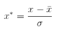
logits:logit的值域范围[-inf,+inf]（即正负无穷区间）。我们可以把logist理解为原生态的、未经缩放的，可视为一种未归一化的l“概率替代物”，如[4, 1, -2]。它可以是其他分类器（如逻辑回归等、SVM等）的输出。

logit公式如下：

                                                                                 

Odds（A）= 发生事件A次数 /  其他事件的次数（即不发生A的次数）

概率P（A）和Odds（A）的值域是不同的。前者被锁定在[0,1]之间，而后者则是[0,∞)

softmax对于logits的用处：

Softmax把一个系列的概率替代物（logits）从[-inf, +inf] 映射到[0,1]

(2)L2损失

l2 = tf.add_n([tf.nn.l2_loss(var) for var in tf.trainable_variables()])

参数解析：

l2_loss:1/2Σvar^2或者output = sum(t ** 2) / 2

L1正则化是指权值向量w中各个元素的绝对值之和，通常表示为||w||1

L2正则化是指权值向量w中各个元素的平方和然后再求平方根（可以看到Ridge回归的L2正则化项有平方符号），通常表示为||w||2  

也就是说Lx范数应用于优化的目标函数就叫做Lx正则化  

l2_loss一般用于优化目标函数中的正则项，防止参数太多复杂容易过拟合(所谓的过拟合问题是指当一个模型很复杂时，它可以很好的“记忆”每一个训练数据中的随机噪声的部分而忘记了要去“学习”训练数据中通用的趋势)

tf.add_n:多个l2(var向量)对应元素相加变为1行var

(3)动量梯度下降算法

train_step = tf.train.MomentumOptimizer(learning_rate, momentum_rate, use_nesterov=True).\
        minimize(cross_entropy + l2 * weight_decay)

参数解析：

learning_rate: （学习率）张量或者浮点数  

momentum: （动量）张量或者浮点数

use_locking: 为True时锁定更新

name: 梯度下降名称，默认为 "Momentum".

use_nesterov:  为True时，使用 Nesterov Momentum

梯度下降法参数更新公式：

W:=W−α∇W

b:=b−α∇b

可以看到，每次更新仅与当前梯度值相关，并不涉及之前的梯度。

而动量梯度下降法则对各个mini-batch求得的梯度∇W,∇b 使用指数加权平均得到 V∇w，V∇b 并使用新的参数更新之前的参数。

例如，在100次梯度下降中求得的梯度序列为:

{∇W1,∇W2,∇W3.........∇W99 ,∇W100}

则其对应的动量梯度分别为：

                                                                      

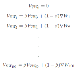
使用指数加权平均之后梯度代替原梯度进行参数更新。

因为每个指数加权平均后的梯度含有之前梯度的信息。

4.准确率

    correct_prediction = tf.equal(tf.argmax(output, 1), tf.argmax(y_, 1))
    accuracy = tf.reduce_mean(tf.cast(correct_prediction, tf.float32))

tf.argmax( , )参数解析：

第一个参数是矩阵，第二个参数是0或者1。 0表示的是按列比较返回最大值的索引， 1表示按行比较返回最大值的索引。 tf.equal(A, B)参数解析：

对比这A和B两个矩阵或者向量的相等的元素， 如果是相等的那就返回True，否则返回False， 返回的值的矩阵维度和A是一样的。

tf.cast(x,dtype)参数解析：

将x的数据格式转化成dtype

例如，原来x的数据格式是bool，那么将其转化成float以后，就能够将其转化成0和1的序列。反之也可以。

五、训练过程和结果

由于一个epoch耗时34s，因此164个epoch需要大约1.5小时训练完成

1.训练过程

2.结果

其中学习率在epoch为82和122时会有转变，代码部分如下：

def learning_rate_schedule(epoch_num):
    if epoch_num < 81:
        return 0.1
    elif epoch_num < 121:
        return 0.01
    else:
        return 0.001

tensorboard结果：

我们也可以从图表中看到在82和121的剧烈变化

最终训练准确率在89%左右，测试准确率在84.5%左右~

六、参考博客和文献

1.2014-VGG-《Very deep convolutional networks for large-scale image recognition》

2.VGG结构的基本理解

3.数据规范化（归一化）、及Z-score标准化

4.tf.nn.softmax_cross_entropy_with_logits中的“logits”到底是个什么意思？

5.tf.nn.l2_loss和 tf.nn.l2_normalize

6.TensorFlow三种常用的优化器

7.动量梯度下降法(gradient descent with momentum)

返回至原博客：vs2017安装和使用教程（详细）