机器学习训练营——机器学习爱好者的自由交流空间(qq 群号:696721295)
分类原理
本例模拟一个多标签文档分类问题。数据集根据下面的过程随机产生。
-
选择标签数
n: 来自泊松分布。 -
选择一个类别
c: 来自多项分布。 -
选择文档长度
k: 来自泊松分布。 -
选择一个单词
w: 来自多项分布。
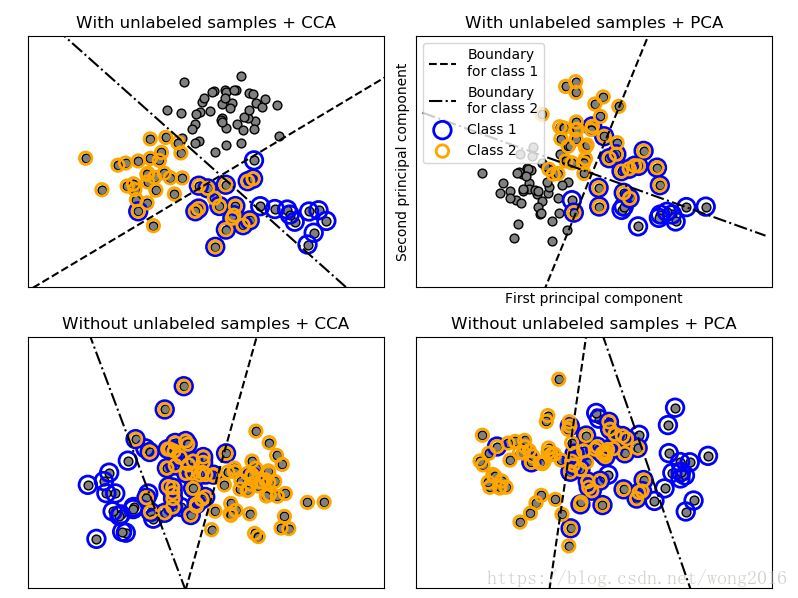
在上述过程里,使用拒绝采样(rejection sampling)确保n>2, 文档长度不是0. 同样地,我们也拒绝已经被选择的类。被分配两个类的文档,在图上用两种颜色圈出。
通过投射到PCA的前两个主成分做分类,然后使用sklearn.multiclass.OneVsRestClassifier分类器学习一个两类的判别模型。请注意,PCA是用来作一个无监督的降维,而CCA(典型关联分析)是用作有监督的降维。不同情况下的样本分类结果见下图。
注意:在下图中,无标签的样本并不意味着我们不能预测它们的标签,而是样本没有标签。
代码详解
首先,在Python环境加载必须的函数库。
print(__doc__)

import numpy as np
import matplotlib.pyplot as plt

from sklearn.datasets import make_multilabel_classification
from sklearn.multiclass import OneVsRestClassifier
from sklearn.svm import SVC
from sklearn.preprocessing import LabelBinarizer
from sklearn.decomposition import PCA
from sklearn.cross_decomposition import CCA
为了在一个图形里同时画四个图,需要定义四个分隔的超平面。为此,定义一个函数plot_hyperplane实现。
def plot_hyperplane(clf, min_x, max_x, linestyle, label):
    # get the separating hyperplane
    w = clf.coef_[0]
    a = -w[0] / w[1]
    xx = np.linspace(min_x - 5, max_x + 5)  # make sure the line is long enough
    yy = a * xx - (clf.intercept_[0]) / w[1]
    plt.plot(xx, yy, linestyle, label=label)
再定义一个函数plot_subfigure, 实现每个超平面内子图的画法。
def plot_subfigure(X, Y, subplot, title, transform):
    if transform == "pca":
        X = PCA(n_components=2).fit_transform(X)
    elif transform == "cca":
        X = CCA(n_components=2).fit(X, Y).transform(X)
    else:
        raise ValueError

    min_x = np.min(X[:, 0])
    max_x = np.max(X[:, 0])

    min_y = np.min(X[:, 1])
    max_y = np.max(X[:, 1])

    classif = OneVsRestClassifier(SVC(kernel='linear'))
    classif.fit(X, Y)

    plt.subplot(2, 2, subplot)
    plt.title(title)

    zero_class = np.where(Y[:, 0])
    one_class = np.where(Y[:, 1])
    plt.scatter(X[:, 0], X[:, 1], s=40, c='gray', edgecolors=(0, 0, 0))
    plt.scatter(X[zero_class, 0], X[zero_class, 1], s=160, edgecolors='b',
                facecolors='none', linewidths=2, label='Class 1')
    plt.scatter(X[one_class, 0], X[one_class, 1], s=80, edgecolors='orange',
                facecolors='none', linewidths=2, label='Class 2')

    plot_hyperplane(classif.estimators_[0], min_x, max_x, 'k--',
                    'Boundary\nfor class 1')
    plot_hyperplane(classif.estimators_[1], min_x, max_x, 'k-.',
                    'Boundary\nfor class 2')
    plt.xticks(())
    plt.yticks(())

    plt.xlim(min_x - .5 * max_x, max_x + .5 * max_x)
    plt.ylim(min_y - .5 * max_y, max_y + .5 * max_y)
    if subplot == 2:
        plt.xlabel('First principal component')
        plt.ylabel('Second principal component')
        plt.legend(loc="upper left")
最后,调用datasets库函数make_multilabel_classification, 在两个主成分类上实现多类别分类,在每个超平面上画出子图。
plt.figure(figsize=(8, 6))

X, Y = make_multilabel_classification(n_classes=2, n_labels=1,
                                      allow_unlabeled=True,
                                      random_state=1)

plot_subfigure(X, Y, 1, "With unlabeled samples + CCA", "cca")
plot_subfigure(X, Y, 2, "With unlabeled samples + PCA", "pca")

X, Y = make_multilabel_classification(n_classes=2, n_labels=1,
                                      allow_unlabeled=False,
                                      random_state=1)

plot_subfigure(X, Y, 3, "Without unlabeled samples + CCA", "cca")
plot_subfigure(X, Y, 4, "Without unlabeled samples + PCA", "pca")

plt.subplots_adjust(.04, .02, .97, .94, .09, .2)
plt.show()
阅读更多精彩内容,请关注微信公众号:统计学习与大数据