原型聚类（二）学习向量量化（LVQ）和python实现

版权声明：本文为博主原创文章，若转载请注明出处。 https://blog.csdn.net/z962013489/article/details/82823932

学习向量量化(Learning Vector Quantization,LVQ)和k-means类似，也属于原型聚类的一种算法，不同的是，LVQ处理的是有标签的样本集，学习过程利用样本的标签进行辅助聚类，个人感觉这个算法更像是一个分类算法。。。

若存在一个样本集 $D=\begin{Bmatrix} (x_{1},y_{1}),(x_{2},y_{2}),...,(x_{m},y_{m}) \end{Bmatrix}$，LVQ希望通过这些样本和标签，学习一组原型向量 $\begin{Bmatrix} p_{1},p_{2},...,p_{q} \end{Bmatrix}$，其中q为样本中的类别总数，算法的思想大概是在初始化原型向量后，根据样本自带的标签让对应的原型向量像该样本靠拢，最终趋于稳定，返回得到的原型向量。

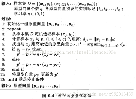
（图片来自《机器学习》周志华

python3.6实现

# -*- coding: gbk -*-

import numpy as np
import copy
from sklearn.datasets import make_moons
from sklearn.datasets.samples_generator import make_blobs
import matplotlib.pyplot as plt


class LVQ():
    def __init__(self, max_iter=10000, eta=0.1, e=0.01):
        self.max_iter = max_iter
        self.eta = eta
        self.e = e

    def dist(self, x1, x2):
        return np.linalg.norm(x1 - x2)

    def get_mu(self, X, Y):
        k = len(set(Y))
        index = np.random.choice(X.shape[0], 1, replace=False)
        mus = []
        mus.append(X[index])
        mus_label = []
        mus_label.append(Y[index])
        for _ in range(k - 1):
            max_dist_index = 0
            max_distance = 0
            for j in range(X.shape[0]):
                min_dist_with_mu = 999999

                for mu in mus:
                    dist_with_mu = self.dist(mu, X[j])
                    if min_dist_with_mu > dist_with_mu:
                        min_dist_with_mu = dist_with_mu

                if max_distance < min_dist_with_mu:
                    max_distance = min_dist_with_mu
                    max_dist_index = j
            mus.append(X[max_dist_index])
            mus_label.append(Y[max_dist_index])

        mus_array = np.array([])
        for i in range(k):
            if i == 0:
                mus_array = mus[i]
            else:
                mus[i] = mus[i].reshape(mus[0].shape)
                mus_array = np.append(mus_array, mus[i], axis=0)
        mus_label_array = np.array(mus_label)
        return mus_array, mus_label_array

    def get_mu_index(self, x):
        min_dist_with_mu = 999999
        index = -1

        for i in range(self.mus_array.shape[0]):
            dist_with_mu = self.dist(self.mus_array[i], x)
            if min_dist_with_mu > dist_with_mu:
                min_dist_with_mu = dist_with_mu
                index = i

        return index

    def fit(self, X, Y):
        self.mus_array, self.mus_label_array = self.get_mu(X, Y)
        iter = 0

        while(iter < self.max_iter):
            old_mus_array = copy.deepcopy(self.mus_array)
            index = np.random.choice(Y.shape[0], 1, replace=False)

            mu_index = self.get_mu_index(X[index])
            if self.mus_label_array[mu_index] == Y[index]:
                self.mus_array[mu_index] = self.mus_array[mu_index] + \
                    self.eta * (X[index] - self.mus_array[mu_index])
            else:
                self.mus_array[mu_index] = self.mus_array[mu_index] - \
                    self.eta * (X[index] - self.mus_array[mu_index])

            diff = 0
            for i in range(self.mus_array.shape[0]):
                diff += np.linalg.norm(self.mus_array[i] - old_mus_array[i])
            if diff < self.e:
                print('迭代{}次退出'.format(iter))
                return
            iter += 1
        print("迭代超过{}次，退出迭代".format(self.max_iter))


if __name__ == '__main__':

    fig = plt.figure(1)

    plt.subplot(221)
    center = [[1, 1], [-1, -1], [1, -1]]
    cluster_std = 0.35
    X1, Y1 = make_blobs(n_samples=1000, centers=center,
                        n_features=2, cluster_std=cluster_std, random_state=1)
    plt.scatter(X1[:, 0], X1[:, 1], marker='o', c=Y1)

    plt.subplot(222)
    lvq1 = LVQ()
    lvq1.fit(X1, Y1)
    mus = lvq1.mus_array
    plt.scatter(X1[:, 0], X1[:, 1], marker='o', c=Y1)
    plt.scatter(mus[:, 0], mus[:, 1], marker='^', c='r')

    plt.subplot(223)
    X2, Y2 = make_moons(n_samples=1000, noise=0.1)
    plt.scatter(X2[:, 0], X2[:, 1], marker='o', c=Y2)

    plt.subplot(224)
    lvq2 = LVQ()
    lvq2.fit(X2, Y2)
    mus = lvq2.mus_array
    plt.scatter(X2[:, 0], X2[:, 1], marker='o', c=Y2)
    plt.scatter(mus[:, 0], mus[:, 1], marker='^', c='r')
    plt.show()

运行返回的原型向量画出如下红色三角：

图中左侧为原始生成的数据，右边红色三角为LVQ聚类获得的原型向量

参考

《机器学习》周志华