将稀疏自编码器与softmax回归结合起来,形成一个简单的三层网络,数据还是mnist,即第一层为28*28个神经元的输入层,中间一个200个神经元的隐藏层,后面再跟一个softmax的5分类loss层。
首先用稀疏自编码的方法无监督训练隐藏层,数据为5-9label的图像,将隐藏层的权值W1训练成下面这样的模式(之前已经做过的):
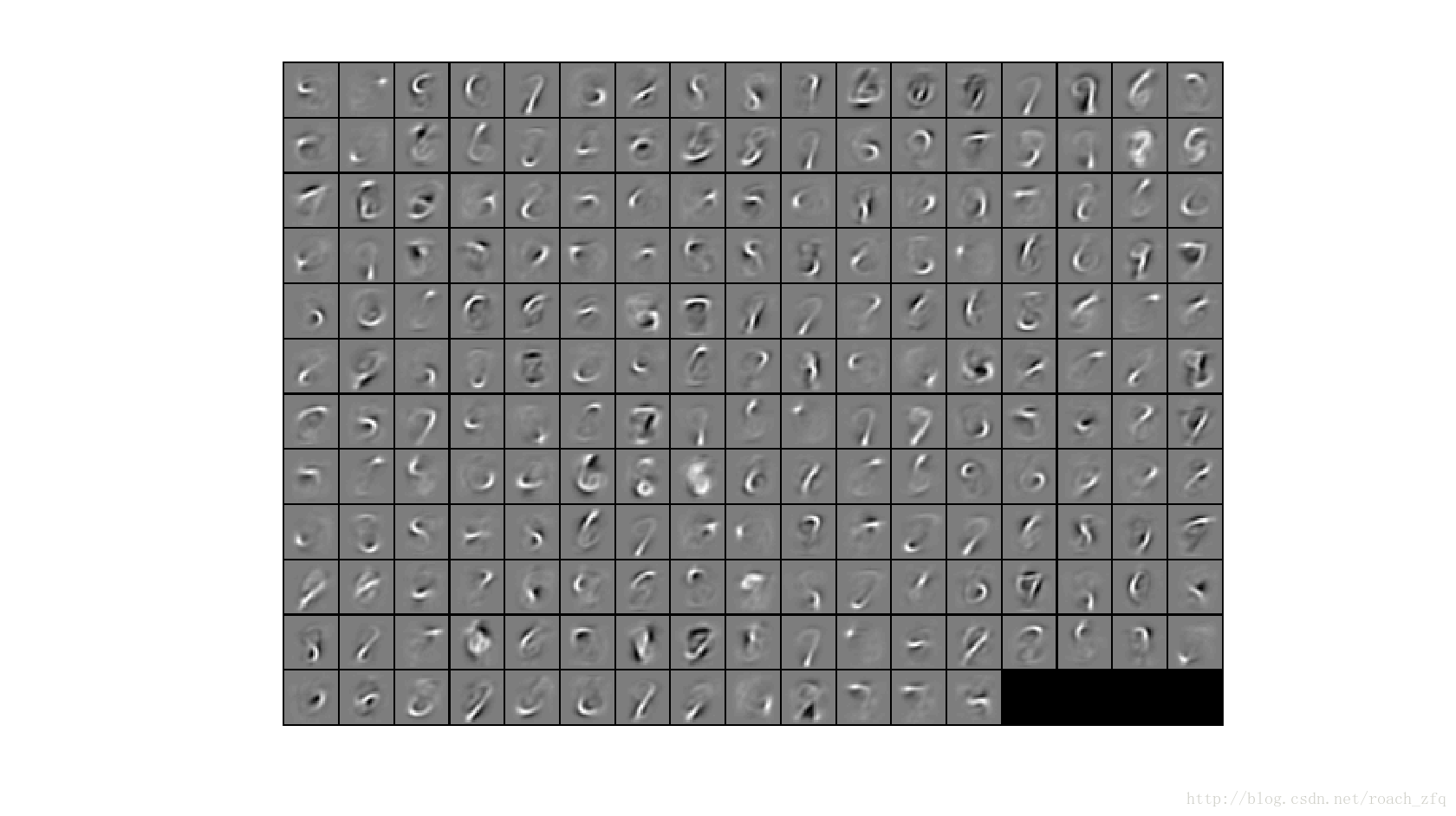
为200张图片,每张图片都是一个神经元的权值按顺序组成的数组可视化后的图片。
有了这些权值W1,保留不变,将0-4label的图像输入,经过与W1相乘后再通过隐藏层sigmoid激活后很快可得到隐藏层的输出,再把这些输出(200*训练图像数量)输入到最后的softmax层进行softmax回归训练,因为只有0-4label,所以softmax为5分类,计算相应的代价函数进行梯度下降训练,得到最后训练好的包含W2的softmaxModel,再用这个model对另一半的测试数据测试,得到准确率。
代码如下:
stlExercise.m
%% CS294A/CS294W Self-taught Learning Exercise

%  Instructions
%  ------------
%
%  This file contains code that helps you get started on the
%  self-taught learning. You will need to complete code in feedForwardAutoencoder.m
%  You will also need to have implemented sparseAutoencoderCost.m and
%  softmaxCost.m from previous exercises.
%
%% ======================================================================
%  STEP 0: Here we provide the relevant parameters values that will
%  allow your sparse autoencoder to get good filters; you do not need to
%  change the parameters below.

clc;
clear;

inputSize  = 28 * 28;
numLabels  = 5;
hiddenSize = 200;
sparsityParam = 0.1; % desired average activation of the hidden units.
                     % (This was denoted by the Greek alphabet rho, which looks like a lower-case "p",
                     %  in the lecture notes).
lambda = 3e-3;       % weight decay parameter
beta = 3;            % weight of sparsity penalty term
maxIter = 400;

%% ======================================================================
%  STEP 1: Load data from the MNIST database
%
%  This loads our training and test data from the MNIST database files.
%  We have sorted the data for you in this so that you will not have to
%  change it.

% Load MNIST database files
mnistData   = loadMNISTImages('mnist/train-images-idx3-ubyte');
mnistLabels = loadMNISTLabels('mnist/train-labels-idx1-ubyte');

% Set Unlabeled Set (All Images)

% Simulate a Labeled and Unlabeled set
labeledSet   = find(mnistLabels >= 0 & mnistLabels <= 4); %符合要求的数字在数组内的下标
unlabeledSet = find(mnistLabels >= 5);

numTrain = round(numel(labeledSet)/2);
trainSet = labeledSet(1:numTrain);      %有label的一半train
testSet  = labeledSet(numTrain+1:end);          %一半test

unlabeledData = mnistData(:, unlabeledSet);

trainData   = mnistData(:, trainSet);   %有label的train data
trainLabels = mnistLabels(trainSet)' + 1; % Shift Labels to the Range 1-5

testData   = mnistData(:, testSet);
testLabels = mnistLabels(testSet)' + 1;   % Shift Labels to the Range 1-5

% Output Some Statistics
fprintf('# examples in unlabeled set: %d\n', size(unlabeledData, 2));
fprintf('# examples in supervised training set: %d\n\n', size(trainData, 2));
fprintf('# examples in supervised testing set: %d\n\n', size(testData, 2));

%% ======================================================================
%  STEP 2: Train the sparse autoencoder
%  This trains the sparse autoencoder on the unlabeled training
%  images.

%% ----------------- YOUR CODE HERE ----------------------
%  Find opttheta by running the sparse autoencoder on
%  unlabeledTrainingImages

%  Randomly initialize the parameters
theta = initializeParameters(hiddenSize, inputSize);

addpath minFunc/
options.Method = 'lbfgs'; % Here, we use L-BFGS to optimize our cost
                          % function. Generally, for minFunc to work, you
                          % need a function pointer with two outputs: the
                          % function value and the gradient. In our problem,
                          % sparseAutoencoderCost.m satisfies this.
options.maxIter = 400;    % Maximum number of iterations of L-BFGS to run
options.display = 'on';


[opttheta, cost] = minFunc( @(p) sparseAutoencoderCost(p, ...
                                   inputSize, hiddenSize, ...
                                   lambda, sparsityParam, ...
                                   beta, unlabeledData), ...
                              theta, options);

%% -----------------------------------------------------

% Visualize weights
W1 = reshape(opttheta(1:hiddenSize * inputSize), hiddenSize, inputSize);
display_network(W1');

%%======================================================================
%% STEP 3: Extract Features from the Supervised Dataset
%
%  You need to complete the code in feedForwardAutoencoder.m so that the
%  following command will extract features from the data.

trainFeatures = feedForwardAutoencoder(opttheta, hiddenSize, inputSize, ...
                                       trainData);  %200*train数据量

testFeatures = feedForwardAutoencoder(opttheta, hiddenSize, inputSize, ...
                                       testData);  %200*test数据量

%%======================================================================
%% STEP 4: Train the softmax classifier

softmaxModel = struct;
%% ----------------- YOUR CODE HERE ----------------------
%  Use softmaxTrain.m from the previous exercise to train a multi-class
%  classifier.

%  Use lambda = 1e-4 for the weight regularization for softmax

% You need to compute softmaxModel using softmaxTrain on trainFeatures and
% trainLabels

lambda = 1e-4;
numClasses = 5;
options.maxIter = 400;
inputSize = hiddenSize;
softmaxModel = softmaxTrain(inputSize, numClasses, lambda, ...
                            trainFeatures, trainLabels, options);

%% -----------------------------------------------------


%%======================================================================
%% STEP 5: Testing

%% ----------------- YOUR CODE HERE ----------------------
% Compute Predictions on the test set (testFeatures) using softmaxPredict
% and softmaxModel
[pred] = softmaxPredict(softmaxModel, testFeatures);

%% -----------------------------------------------------
% Classification Score
fprintf('Test Accuracy: %f%%\n', 100*mean(pred(:) == testLabels(:)));

% (note that we shift the labels by 1, so that digit 0 now corresponds to
%  label 1)
%
% Accuracy is the proportion of correctly classified images
% The results for our implementation was:
%
% Accuracy: 98.3%
%
%
sparseAutoencoderCost.m
function [cost,grad] = sparseAutoencoderCost(theta, visibleSize, hiddenSize, ...
                                             lambda, sparsityParam, beta, data)

% visibleSize: the number of input units (probably 64)
% hiddenSize: the number of hidden units (probably 25)
% lambda: weight decay parameter
% sparsityParam: The desired average activation for the hidden units (denoted in the lecture
%                           notes by the greek alphabet rho, which looks like a lower-case "p").
% beta: weight of sparsity penalty term
% data: Our 64x10000 matrix containing the training data.  So, data(:,i) is the i-th training example.

% The input theta is a vector (because minFunc expects the parameters to be a vector).
% We first convert theta to the (W1, W2, b1, b2) matrix/vector format, so that this
% follows the notation convention of the lecture notes.

W1 = reshape(theta(1:hiddenSize*visibleSize), hiddenSize, visibleSize);
W2 = reshape(theta(hiddenSize*visibleSize+1:2*hiddenSize*visibleSize), visibleSize, hiddenSize);
b1 = theta(2*hiddenSize*visibleSize+1:2*hiddenSize*visibleSize+hiddenSize);
b2 = theta(2*hiddenSize*visibleSize+hiddenSize+1:end);

% Cost and gradient variables (your code needs to compute these values).
% Here, we initialize them to zeros.
cost = 0;

%% ---------- YOUR CODE HERE --------------------------------------
%  Instructions: Compute the cost/optimization objective J_sparse(W,b) for the Sparse Autoencoder,
%                and the corresponding gradients W1grad, W2grad, b1grad, b2grad.
%
% W1grad, W2grad, b1grad and b2grad should be computed using backpropagation.
% Note that W1grad has the same dimensions as W1, b1grad has the same dimensions
% as b1, etc.  Your code should set W1grad to be the partial derivative of J_sparse(W,b) with
% respect to W1.  I.e., W1grad(i,j) should be the partial derivative of J_sparse(W,b)
% with respect to the input parameter W1(i,j).  Thus, W1grad should be equal to the term
% [(1/m) \Delta W^{(1)} + \lambda W^{(1)}] in the last block of pseudo-code in Section 2.2
% of the lecture notes (and similarly for W2grad, b1grad, b2grad).
%
% Stated differently, if we were using batch gradient descent to optimize the parameters,
% the gradient descent update to W1 would be W1 := W1 - alpha * W1grad, and similarly for W2, b1, b2.
%
numPatches = size(data,2);
KLdist = 0;

z2 = W1 * data + repmat(b1,[1,numPatches]);   %25*10000
a2 = sigmoid(z2);                         %25*10000
p = sum(a2,2);                 %25*1
z3 = W2 * a2 + repmat(b2,[1,numPatches]); %64*10000
a3 = sigmoid(z3);                          %64*10000
J_sparse = 0.5 * sum(sum((a3-data).^2));

p = p / numPatches;   %计算隐藏层的平均激活度

%% 向后传输
residual3 = -(data-a3).*a3.*(1-a3);  %残差公式 %64x10000
tmp = beta * ( - sparsityParam ./ p + (1-sparsityParam) ./ (1-p)); %25*1
%  25x10000   25x64 64x10000
residual2 = (W2' * residual3 + repmat(tmp,[1,numPatches])) .* a2.*(1-a2);
W2grad = residual3 * a2' / numPatches + lambda * W2 ;  %64*25
W1grad = residual2 * data'  / numPatches + lambda * W1 ;%25*64
b2grad = sum(residual3,2) / numPatches; %64*1
b1grad = sum(residual2,2) / numPatches; %25*1

%% 计算KL相对熵
for j = 1:hiddenSize
    KLdist = KLdist + sparsityParam *log( sparsityParam / p(j) )   +   (1 - sparsityParam) * log((1-sparsityParam) / (1 - p(j)));
end

cost = J_sparse / numPatches + (sum(sum(W1.^2)) + sum(sum(W2.^2))) * lambda / 2  + beta * KLdist;

%-------------------------------------------------------------------
% After computing the cost and gradient, we will convert the gradients back
% to a vector format (suitable for minFunc).  Specifically, we will unroll
% your gradient matrices into a vector.

grad = [W1grad(:) ; W2grad(:) ; b1grad(:) ; b2grad(:)];

end

%-------------------------------------------------------------------
% Here's an implementation of the sigmoid function, which you may find useful
% in your computation of the costs and the gradients.  This inputs a (row or
% column) vector (say (z1, z2, z3)) and returns (f(z1), f(z2), f(z3)).

function sigm = sigmoid(x)

    sigm = 1 ./ (1 + exp(-x));
end
softmaxCost.m
function [cost, grad] = softmaxCost(theta, numClasses, inputSize, lambda, data, labels)

% numClasses - the number of classes
% inputSize - the size N of the input vector
% lambda - weight decay parameter
% data - the N x M input matrix, where each column data(:, i) corresponds to
%        a single test set
% labels - an M x 1 matrix containing the labels corresponding for the input data
%

% Unroll the parameters from theta
theta = reshape(theta, numClasses, inputSize); %10*784

numCases = size(data, 2);   %60000

groundTruth = full(sparse(labels, 1:numCases, 1));  %10*60000
cost = 0;

thetagrad = zeros(numClasses, inputSize);

%% ---------- YOUR CODE HERE --------------------------------------
%  Instructions: Compute the cost and gradient for softmax regression.
%                You need to compute thetagrad and cost.
%                The groundTruth matrix might come in handy.

thetaTx = theta * data;   % 10*60000
%减去最大值 防止exp值过大溢出
thetaTx = bsxfun(@minus, thetaTx, max(thetaTx, [], 1));   % 10*60000
eThetaTx = exp(thetaTx);   % 10*60000
hypothesis = eThetaTx./(repmat(sum(eThetaTx),size(eThetaTx,1),1)); % 10*60000

cost = -sum(sum(log(hypothesis).*groundTruth))/numCases;
cost = cost + sum(sum(theta.^2))*lambda/2;

thetagrad = -(groundTruth - hypothesis)*data'./numCases + lambda.*theta;  %10*784

% ------------------------------------------------------------------
% Unroll the gradient matrices into a vector for minFunc
grad = [thetagrad(:)];
end
feedForwardAutoencoder.m
function [activation] = feedForwardAutoencoder(theta, hiddenSize, visibleSize, data)

% theta: trained weights from the autoencoder
% visibleSize: the number of input units (probably 784)
% hiddenSize: the number of hidden units (probably 200)
% data: Our matrix containing the training data as columns.  So, data(:,i) is the i-th training example.

% We first convert theta to the (W1, W2, b1, b2) matrix/vector format, so that this
% follows the notation convention of the lecture notes.

%% ---------- YOUR CODE HERE --------------------------------------
%  Instructions: Compute the activation of the hidden layer for the Sparse Autoencoder.

W1 = reshape(theta(1:hiddenSize*visibleSize), hiddenSize, visibleSize);  %200*784
b1 = theta(2*hiddenSize*visibleSize+1:2*hiddenSize*visibleSize+hiddenSize); %200*1

activation = sigmoid(W1 * data + repmat(b1,[1,size(data,2)]));  %200*15000..

%-------------------------------------------------------------------

end

%-------------------------------------------------------------------
% Here's an implementation of the sigmoid function, which you may find useful
% in your computation of the costs and the gradients.  This inputs a (row or
% column) vector (say (z1, z2, z3)) and returns (f(z1), f(z2), f(z3)).

function sigm = sigmoid(x)
    sigm = 1 ./ (1 + exp(-x));
end
主要就是这几个文件,其余的其他文章里也都提到了,基本上就是把前两章的内容结合起来而已。
运行结果如下:
examples in unlabeled set: 29404
examples in supervised training set: 15298
examples in supervised testing set: 15298
Iteration FunEvals Step Length Function Val Opt Cond
1 5 3.14777e-02 1.10167e+02 8.54784e+03
2 6 1.00000e+00 9.14035e+01 4.37969e+03
3 7 1.00000e+00 8.38713e+01 1.98396e+03
4 8 1.00000e+00 7.95523e+01 2.03865e+03
5 9 1.00000e+00 7.12491e+01 2.72443e+03
6 10 1.00000e+00 5.43268e+01 2.97157e+03
7 11 1.00000e+00 3.28241e+01 8.45774e+02
8 ….
…
…
…
387 398 1.00000e+00 1.16473e+01 5.81143e+00
388 399 1.00000e+00 1.16468e+01 7.29393e+00
389 400 1.00000e+00 1.16462e+01 9.87254e+00
390 401 1.00000e+00 1.16455e+01 8.87469e+00
391 402 1.00000e+00 1.16451e+01 6.20162e+00
392 403 1.00000e+00 1.16445e+01 5.85851e+00
393 404 1.00000e+00 1.16442e+01 6.73153e+00
394 405 1.00000e+00 1.16436e+01 7.44381e+00
395 406 1.00000e+00 1.16433e+01 1.08066e+01
396 407 1.00000e+00 1.16426e+01 6.51165e+00
397 408 1.00000e+00 1.16423e+01 5.74701e+00
398 409 1.00000e+00 1.16419e+01 6.52625e+00
399 410 1.00000e+00 1.16415e+01 6.77704e+00
400 411 1.00000e+00 1.16411e+01 8.99886e+00
Exceeded Maximum Number of Iterations
Iteration FunEvals Step Length Function Val Opt Cond
1 3 6.30893e-01 1.33252e+00 1.33745e+01
2 4 1.00000e+00 4.75012e-01 4.63605e+00
3 5 1.00000e+00 3.35942e-01 3.22785e+00
4 6 1.00000e+00 2.52347e-01 1.51473e+00
5 7 1.00000e+00 1.99355e-01 8.24715e-01
6 8 1.00000e+00 1.65120e-01 9.29615e-01
7 9 1.00000e+00 1.38252e-01 5.01888e-01
8 10 1.00000e+00 1.28380e-01 3.52842e-01
9 11 1.00000e+00 1.14536e-01 2.63068e-01
10 12 1.00000e+00 1.00907e-01 3.94667e-01
11 13 1.00000e+00 9.30330e-02 2.36750e-01
12 14 1.00000e+00 8.75129e-02 1.66041e-01
13 15 1.00000e+00 8.30299e-02 1.09462e-01
14 16 1.00000e+00 7.91959e-02 1.07245e-01
15 17 1.00000e+00 7.65056e-02 1.08345e-01
16 18 1.00000e+00 7.50167e-02 1.22889e-01
17 19 1.00000e+00 7.35633e-02 6.50477e-02
18 20 1.00000e+00 7.28726e-02 4.92305e-02
19 21 1.00000e+00 7.23238e-02 4.84382e-02
20 22 1.00000e+00 7.18056e-02 5.33487e-02
21 23 1.00000e+00 7.13970e-02 5.01899e-02
22 24 1.00000e+00 7.11652e-02 3.17180e-02
23 25 1.00000e+00 7.09514e-02 2.80332e-02
24 26 1.00000e+00 7.08163e-02 2.81097e-02
25 27 1.00000e+00 7.06447e-02 2.41427e-02
26 28 1.00000e+00 7.05202e-02 1.79102e-02
27 29 1.00000e+00 7.04211e-02 1.02507e-02
28 30 1.00000e+00 7.03787e-02 1.20261e-02
29 31 1.00000e+00 7.03509e-02 1.02202e-02
30 32 1.00000e+00 7.03269e-02 8.55803e-03
31 33 1.00000e+00 7.03047e-02 6.39926e-03
32 34 1.00000e+00 7.02937e-02 4.76259e-03
33 35 1.00000e+00 7.02883e-02 3.95992e-03
34 36 1.00000e+00 7.02837e-02 3.65665e-03
35 37 1.00000e+00 7.02802e-02 3.33861e-03
36 38 1.00000e+00 7.02776e-02 2.33751e-03
37 39 1.00000e+00 7.02764e-02 1.37919e-03
38 40 1.00000e+00 7.02755e-02 1.25428e-03
39 41 1.00000e+00 7.02747e-02 1.19318e-03
40 42 1.00000e+00 7.02741e-02 1.35342e-03
41 43 1.00000e+00 7.02738e-02 9.47215e-04
42 44 1.00000e+00 7.02736e-02 4.93086e-04
43 45 1.00000e+00 7.02735e-02 3.68544e-04
44 46 1.00000e+00 7.02734e-02 3.88469e-04
45 47 1.00000e+00 7.02733e-02 3.51496e-04
46 49 4.74595e-01 7.02733e-02 4.15585e-04
47 50 1.00000e+00 7.02733e-02 2.27196e-04
48 51 1.00000e+00 7.02733e-02 1.46213e-04
49 52 1.00000e+00 7.02733e-02 1.18617e-04
50 53 1.00000e+00 7.02733e-02 1.00106e-04
51 54 1.00000e+00 7.02733e-02 7.27407e-05
52 56 3.17967e-01 7.02732e-02 5.64051e-05
53 57 1.00000e+00 7.02732e-02 3.64929e-05
Function Value changing by less than TolX
Test Accuracy: 98.339652%
结果还是和标准答案一模一样啊(确实Ng做的教程相当好,自己完成的代码只有十几行,简单易操作,却都是最关键最能学到东西的地方)
有一点需要在意的就是训练时,稀疏自编码器的训练相当耗时,也就是W1的训练,花了有10分钟,也不知道为什么,意外地长。。然后display了W1的权值图像后(也就是最上面那幅)1秒钟就完成了softmax的训练和测试,\(⊙o⊙)//。。。。可以看到迭代53次后就达到目标loss了,而之前没有加中间的稀疏自编码层时,也就是直接输入28*28个,输出10个,大概350次(也运行相当久)才达到目标。由此可见无监督学习到的特征再与有监督学习结合起来(术语叫半监督学习?)的效果在数据集比较小的情况下确实很有用啊!
最后基本上只用了3层10min便得到98%的准确率,比在caffe上跑的cnn简单太多,耗时又少,虽然准确率还是要差一些的。。