一,课题研究与背景介绍:
1,课题研究:
利用信用卡历史数据进行机器建模,构建反欺诈模型,预测新的信用卡被盗刷的可能性。
2,背景介绍:
数据集包含由欧洲人于2013年9月使用信用卡进行交易的数据。此数据集显示两天内发生的交易,其中284807笔交易中有492笔被盗刷。数据集非常不平衡,正例(被盗刷)占所有交易的0.172%。,这是因为由于保密问题,我们无法提供有关数据的原始功能和更多背景信息。特征V1,V2,... V28是使用PCA获得的主要组件,没有用PCA转换的唯一特征是“Class”和“Amount”。特征'Time'包含数据集中每个刷卡时间和第一次刷卡时间之间经过的秒数。特征'Class'是响应变量,如果发生被盗刷,则取值1,否则为0。
二,数据
1,数据源:https://www.kesci.com/home/dataset/5b56a592fc7e9000103c0442/files
2,用到的库:
Numpy-科学计算库 主要用来做矩阵运算,什么?你不知道哪里会用到矩阵,那么这样想吧,咱们的数据就是行(样本)和列(特征)组成的,那么数据本身不就是一个矩阵嘛。
Pandas-数据分析处理库 很多小伙伴都在说用python处理数据很容易,那么容易在哪呢?其实有了pandas很复杂的操作我们也可以一行代码去解决掉!
Matplotlib-可视化库 无论是分析还是建模,光靠好记性可不行,很有必要把结果和过程可视化的展示出来。
Scikit-Learn-机器学习库 非常实用的机器学习算法库,这里面包含了基本你觉得你能用上所有机器学习算法啦。但还远不止如此,还有很多预处理和评估的模块等你来挖掘的!
三,提出问题:
四,数据预处理:
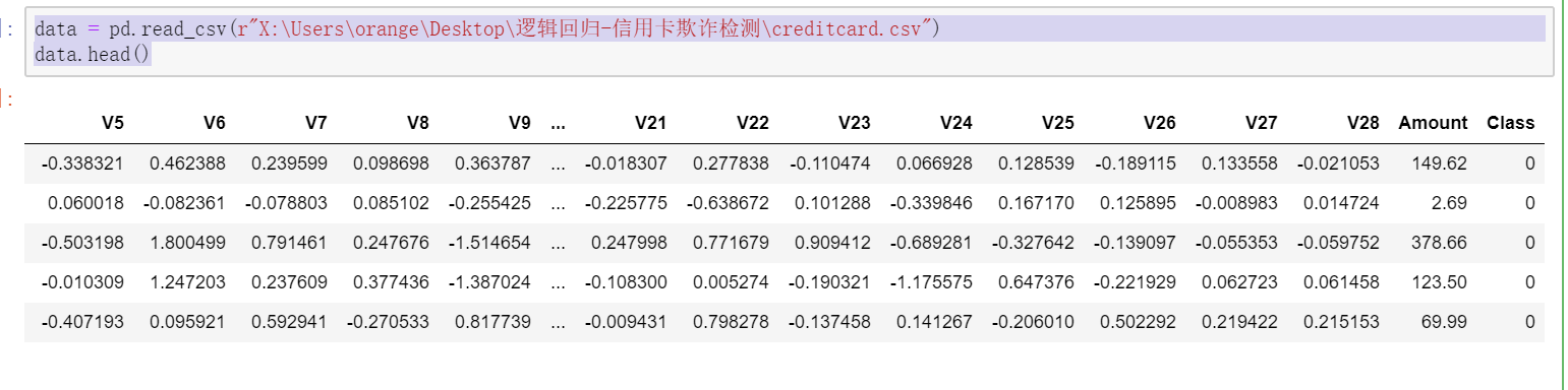
1,读取数据与分析。由于是网站竞赛的数据,所以原作者处于保密性对原数据进行了PCA降维操作,同时也对每个列字段名进行了保密,因此我们在分析过程中不需可以强调每一列的含义。同时数据经过了一系列的数据预处理操作,使得数据比较干净、整洁。class为0是正常的行为,为1是欺诈行为。
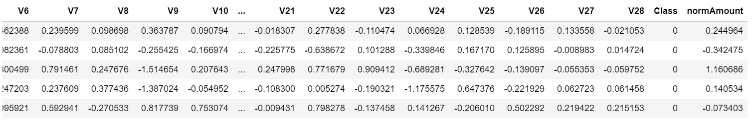
data = pd.read_csv(r"X:\Users\orange\Desktop\逻辑回归-信用卡欺诈检测\creditcard.csv")
data.head()
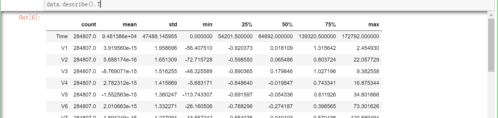
2,查看数据信息:从上面可以看出,数据为结构化数据,不需要抽特征转化,但特征Amount的数据规格和其他特征不一样,需要对其做特征做特征缩放。
data.describe().T
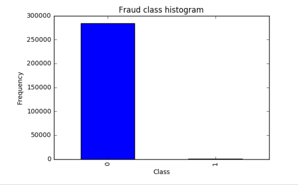
3,正常数据与异常数据的数量差异
在上图中Class标签代表数据分类,0代表正常数据,1代表欺诈数据。
这里是做信用卡数据的欺诈检测。在整个数据里面,有正常的数据,也有问题的数据。对于一般情况来说,有问题的数据肯定只占了极少部分。
下面绘出柱状图可以直观显示正常数据与异常数据的数量差异。
count_classes = pd.value_counts(data['Class'], sort=True).sort_index()
count_classes.plot(kind='bar') # 使用pandas可以绘制一些简单的图
# 欺诈类别柱状图
plt.title("Fraud class histogram")
plt.xlabel("Class")
# 频率
plt.ylabel("Frequency")
4,预处理:标准化数据
从输出的结果可以看出正常的样本0大概有28万个,异常的样本1非常少,从图中不太容易看出来,但是实际上是存在的,大概只有那么几百个。
因为Amount这列的数据浮动太大,在做机器学习的过程中,需要保证特征值差异不能过大,于是需要对Amount进行预处理,标准化数据。
Time这一列本身没有多大用处,Amount这一列被标准化后的数据代替。所有删除这两列的数据。
# 预处理  标准化数据
from sklearn.preprocessing import StandardScaler
# norm 标准  -1表示自动判断X维度  对比源码 这里要加上.values<br># 加上新的特征列
data['normAmount'] = StandardScaler().fit_transform(data['Amount'].values.reshape(-1, 1))
data = data.drop(['Time', 'Amount'], axis=1)
data.head()
 五,样本数据分布不均衡解决方案
1,下采样策略
上面说到数据集里面正常数据和异常数据数量差异极大,对于这种样本数据不均衡问题,一般有以下两种策略:
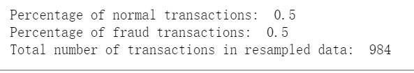
(1)下采样策略:之前统计的结果可以看出0的样本有28万个,而1的样本只有几百个。现在将0的数据也变成几百个就可以了。下采样,是使样本的数据同样少
(2)过采样策略:之前统计的结果可以看出0的样本有28万个,而1的样本只有几百个。0比较多1比较少,对1的样本数据进行生成数列,让生成的数据与0的样本数据一样多。
下面首先采用下采样策略
X = data.ix[:, data.columns != 'Class']
y = data.ix[:, data.columns == 'Class']

# 少数类中的数据点数量
number_records_fraud = len(data[data.Class == 1])
fraud_indices = np.array(data[data.Class == 1].index)

# 选择正常类的指标
normal_indices = data[data.Class == 0].index

# 从我们选择的指数中,随机选择“x”号(number_records_fraud)
random_normal_indices = np.random.choice(normal_indices, number_records_fraud, replace = False)
random_normal_indices = np.array(random_normal_indices)

# 附加两个索引
under_sample_indices = np.concatenate([fraud_indices,random_normal_indices])

# 在样本数据集
under_sample_data = data.iloc[under_sample_indices,:]

X_undersample = under_sample_data.ix[:, under_sample_data.columns != 'Class']
y_undersample = under_sample_data.ix[:, under_sample_data.columns == 'Class']

# 显示比例
print("Percentage of normal transactions: ", len(under_sample_data[under_sample_data.Class == 0])/len(under_sample_data))
print("Percentage of fraud transactions: ", len(under_sample_data[under_sample_data.Class == 1])/len(under_sample_data))
print("Total number of transactions in resampled data: ", len(under_sample_data))
2,切分数据
可以看出经过下采样策略过后,正常数据与异常数据各占50%,并且总样本数也只有少部分。
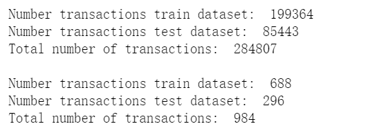
下面对原始数据集和下采样后的数据集分别进行切分操作。
from sklearn.cross_validation import train_test_split

# 整个数据集
X_train, X_test, y_train, y_test = train_
test_split(X,y,test_size = 0.3, random_state = 0)

print("Number transactions train dataset: ", len(X_train))
print("Number transactions test dataset: ", len(X_test))
print("Total number of transactions: ", len(X_train)+len(X_test))

# Undersampled数据集
X_train_undersample, X_test_undersample, y_train_undersample, y_test_undersample = train_test_split(X_undersample
                                                                                                   ,y_undersample
                                                                                                   ,test_size = 0.3
                                                                                                   ,random_state = 0)
print("")
print("Number transactions train dataset: ", len(X_train_undersample))
print("Number transactions test dataset: ", len(X_test_undersample))
print("Total number of transactions: ", len(X_train_undersample)+len(X_test_undersample))
六,交叉验证
比如有个集合叫data,通常建立机器模型的时候,先对数据进行切分或者选择,取前面80%的数据当成训练集,取20%的数据当成测试集。80%的数据是来建立一个模型,剩下的20%的数据是用来测试模型。因此第一步是将数据进行切分,切分成训练集以及测试集。这部分操作是必须要做的。第二步还要在训练集进行平均切分,比如平均切分成3份,分别是数据集1,2,3。
在建立模型的时候,不管建立什么样的模型,这个模型伴随着很多参数,有不同的参数进行选择,这个参数选择大比较好,还是选择小比较好一些?从经验值角度来说,肯定没办法很准的,怎么样去确定这个参数呢?只能通过交叉验证的方式。
那什么又叫交叉验证呢?
第一次:将数据集1,2分别建立模型,用数据集3在当前权重下去验证当前模型的效果。数据集3是个验证集,验证集是训练集的一部分。用验证集去验证模型是好还是坏。
第二次:将数据集1,3分别建立模型,用数据集2在当前权重下去验证当前模型的效果。
第三次:将数据集2,3分别建立模型,用数据集1在当前权重下去验证当前模型的效果。
如果只是求一次的交叉验证,这样的操作会存在风险。比如只做第一次交叉验证,会使3验证集偏简单一些。会使模型效果偏高,此外模型有些数据是错误值以及离群值,如果把这些不太好的数据当成验证集,会使模型的效果偏低的。模型当然是不希望偏高也不希望偏低,那就需要多做几次交叉验证模型,求平均值。这里有1,2,3分别作验证集,每个验证集都有评估的标准。最终模型的效果将1,2,3的评估效果加在一起,再除以3,就可以得到模型一个大致的效果。
#Recall = TP/(TP+FN)
from sklearn.linear_model import LogisticRegression
from sklearn.cross_validation import KFold, cross_val_score
from sklearn.metrics import confusion_matrix,recall_score,classification_report
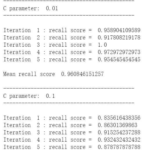
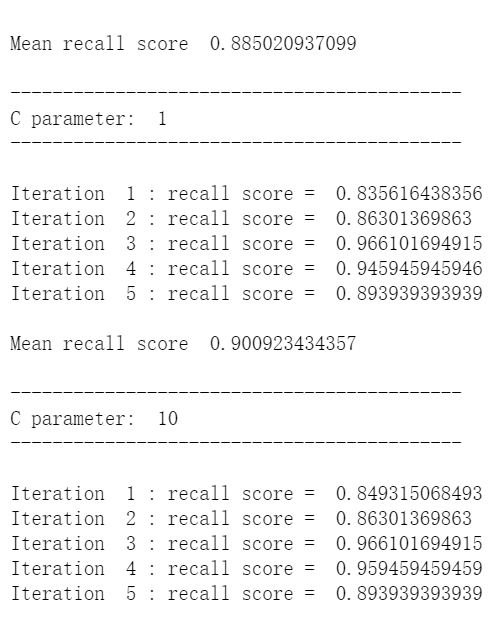
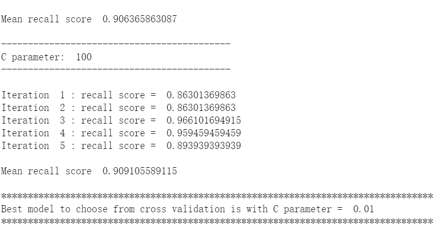
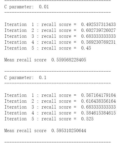
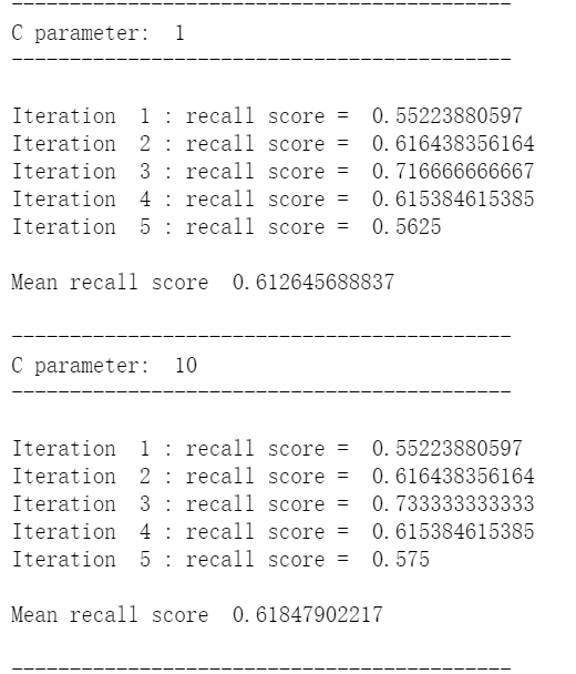
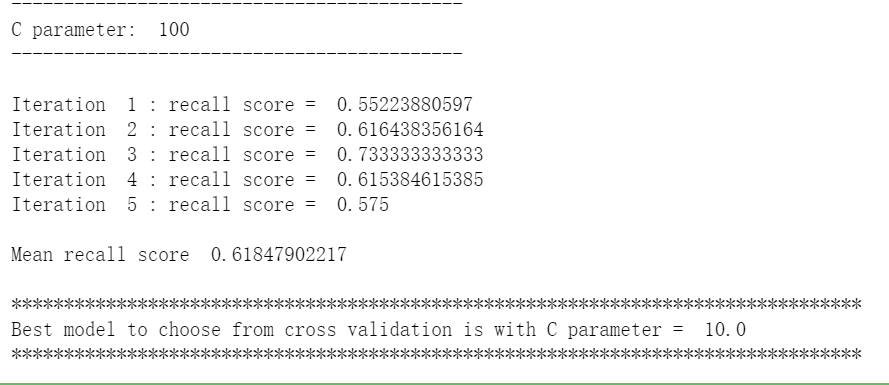
def printing_Kfold_scores(x_train_data,y_train_data):
    fold = KFold(len(y_train_data),5,shuffle=False)

    # 不同的C参数
    c_param_range = [0.01,0.1,1,10,100]

    results_table = pd.DataFrame(index = range(len(c_param_range),2), columns = ['C_parameter','Mean recall score'])
    results_table['C_parameter'] = c_param_range

    # k-fold将给出2个列表:train_indices = indices[0], test_indices = indices[1]
    j = 0
    for c_param in c_param_range:
        print('-------------------------------------------')
        print('C parameter: ', c_param)
        print('-------------------------------------------')
        print('')

        recall_accs = []
        for iteration, indices in enumerate(fold,start=1):

            # 调用具有特定C参数的logistic回归模型
            lr = LogisticRegression(C = c_param, penalty = 'l1')

            # 使用训练数据来拟合模型。在本例中,我们使用折叠的部分来训练模型
            # 与指数[0]。然后,我们使用索引[1]预测指定为“测试交叉验证”的部分
            lr.fit(x_train_data.iloc[indices[0],:],y_train_data.iloc[indices[0],:].values.ravel())

            # 利用训练数据中的测试指标预测值
            y_pred_undersample = lr.predict(x_train_data.iloc[indices[1],:].values)

            # 计算收回分数,并将其追加到表示当前c_parameter的收回分数的列表中
            recall_acc = recall_score(y_train_data.iloc[indices[1],:].values,y_pred_undersample)
            recall_accs.append(recall_acc)
            print('Iteration ', iteration,': recall score = ', recall_acc)

        # 这些回忆分数的平均值是我们想要保存和获得的度量标准。
        results_table.ix[j,'Mean recall score'] = np.mean(recall_accs)
        j += 1
        print('')
        print('Mean recall score ', np.mean(recall_accs))
        print('')

    best_c = results_table.loc[results_table['Mean recall score'].idxmax()]['C_parameter']

    # 最后,我们可以检查所选的C参数中哪个是最好的。
    print('*********************************************************************************')
    print('Best model to choose from cross validation is with C parameter = ', best_c)
    print('*********************************************************************************')

    return best_c
使用下采样数据集调用上面这个函数
best_c = printing_Kfold_scores(X_train_undersample,y_train_undersample)
七,构建矩阵
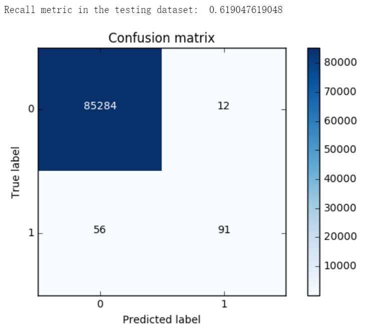
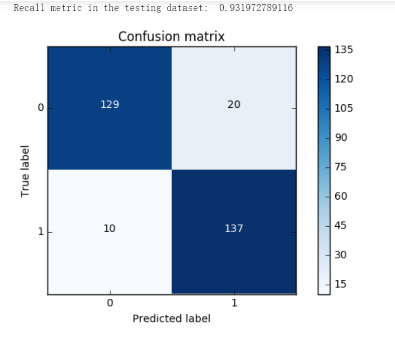
一般都是用精度来衡量,也就是常说的准确率,但是我们来想一想,我们的目的是什么呢?是不是要检测出来那些异常的样本呀!换个例子来说,假如现在医院给了我们一个任务要检测出来1000个病人中,有癌症的那些人。那么假设数据集中1000个人中有990个无癌症,只有10个有癌症,我们需要把这10个人检测出来。假设我们用精度来衡量,那么即便这10个人没检测出来,也是有 990/1000 也就是99%的精度,但是这个模型却没任何价值!这点是非常重要的,因为不同的评估方法会得出不同的答案,一定要根据问题的本质,去选择最合适的评估方法。
同样的道理,这里我们采用recall来计算模型的好坏,也就是说那些异常的样本我们的检测到了多少,这也是咱们最初的目的!这里通常用混淆矩阵来展示。
def plot_confusion_matrix(cm, classes,
                          title='Confusion matrix',
                          cmap=plt.cm.Blues):
    """
    This function prints and plots the confusion matrix.
    """
    plt.imshow(cm, interpolation='nearest', cmap=cmap)
    plt.title(title)
    plt.colorbar()
    tick_marks = np.arange(len(classes))
    plt.xticks(tick_marks, classes, rotation=0)
    plt.yticks(tick_marks, classes)

    thresh = cm.max() / 2.
    for i, j in itertools.product(range(cm.shape[0]), range(cm.shape[1])):
        plt.text(j, i, cm[i, j],
                 horizontalalignment="center",
                 color="white" if cm[i, j] > thresh else "black")

    plt.tight_layout()
    plt.ylabel('True label')
    plt.xlabel('Predicted label')
import itertools
lr = LogisticRegression(C = best_c, penalty = 'l1')
lr.fit(X_train_undersample,y_train_undersample.values.ravel())
y_pred_undersample = lr.predict(X_test_undersample.values)

# Compute confusion matrix
cnf_matrix = confusion_matrix(y_test_undersample,y_pred_undersample)
np.set_printoptions(precision=2)

print("Recall metric in the testing dataset: ", cnf_matrix[1,1]/(cnf_matrix[1,0]+cnf_matrix[1,1]))

# Plot non-normalized confusion matrix
class_names = [0,1]
plt.figure()
plot_confusion_matrix(cnf_matrix
                      , classes=class_names
                      , title='Confusion matrix')
plt.show()
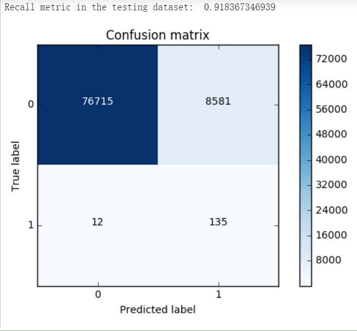
lr = LogisticRegression(C = best_c, penalty = 'l1')
lr.fit(X_train_undersample,y_train_undersample.values.ravel())
y_pred = lr.predict(X_test.values)

# Compute confusion matrix
cnf_matrix = confusion_matrix(y_test,y_pred)
np.set_printoptions(precision=2)

print("Recall metric in the testing dataset: ", cnf_matrix[1,1]/(cnf_matrix[1,0]+cnf_matrix[1,1]))

# Plot non-normalized confusion matrix
class_names = [0,1]
plt.figure()
plot_confusion_matrix(cnf_matrix
                      , classes=class_names
                      , title='Confusion matrix')
plt.show()
继续调用下采样数据集调用上面这个函数
best_c = printing_Kfold_scores(X_train,y_train)
lr = LogisticRegression(C = best_c, penalty = 'l1')
lr.fit(X_train,y_train.values.ravel())
y_pred_undersample = lr.predict(X_test.values)

# Compute confusion matrix
cnf_matrix = confusion_matrix(y_test,y_pred_undersample)
np.set_printoptions(precision=2)

print("Recall metric in the testing dataset: ", cnf_matrix[1,1]/(cnf_matrix[1,0]+cnf_matrix[1,1]))

# Plot non-normalized confusion matrix
class_names = [0,1]
plt.figure()
plot_confusion_matrix(cnf_matrix
                      , classes=class_names
                      , title='Confusion matrix')
plt.show()