                                        <div class="markdown_views">
            <h2 id="前言"><a name="t0"></a>前言</h2>
Tensorflow中可以使用tensorboard这个强大的工具对计算图、loss、网络参数等进行可视化。本文并不涉及对tensorboard使用的介绍,而是旨在说明如何通过代码对网络权值和feature map做更灵活的处理、显示和存储。本文的相关代码主要参考了github上的一个小项目,但是对其进行了改进。原项目地址为(https://github.com/grishasergei/conviz)。
本文将从以下两个方面进行介绍:
- 卷积知识补充
- 网络权值和feature map的可视化
1. 卷积知识补充
为了后面方便讲解代码,这里先对卷积的部分知识进行一下简介。关于卷积核如何在图像的一个通道上进行滑动计算,网上有诸多资料,相信对卷积神经网络有一定了解的读者都应该比较清楚,本文就不再赘述。这里主要介绍一组卷积核如何在一幅图像上计算得到一组feature map。
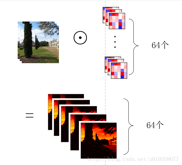
以从原始图像经过第一个卷积层得到第一组feature map为例(从得到的feature map到再之后的feature map也是同理),假设第一组feature map共有64个,那么可以把这组feature map也看作一幅图像,只不过它的通道数是64, 而一般意义上的图像是RGB3个通道。为了得到这第一组feature map,我们需要64个卷积核,每个卷积核是一个k x k x 3的矩阵,其中k是卷积核的大小(假设是正方形卷积核),3就对应着输入图像的通道数。下面我以一个简单粗糙的图示来展示一下图像经过一个卷积核的卷积得到一个feature map的过程。

如图所示,其实可以看做卷积核的每一通道(不太准确,将就一下)和图像的每一通道对应进行卷积操作,然后再逐位置相加,便得到了一个feature map。
那么用一组(64个)卷积核去卷积一幅图像,得到64个feature map就如下图所示,也就是每个卷积核得到一个feature map,64个卷积核就得到64个feature map。
另外,也可以稍微换一个角度看待这个问题,那就是先让图片的某一通道分别与64个卷积核的对应通道做卷积,得到64个feature map的中间结果,之后3个通道对应的中间结果再相加,得到最终的feature map,如下图所示:
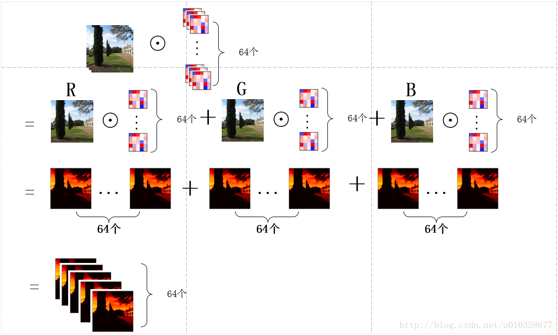
可以看到这其实就是第一幅图扩展到多卷积核的情形,图画得较为粗糙,有些中间结果和最终结果直接用了一样的子图,理解时请稍微注意一下。下面代码中对卷积核进行展示的时候使用的就是这种方式,即对应着输入图像逐通道的去显示卷积核的对应通道,而不是每次显示一个卷积核的所有通道,可能解释的有点绕,需要注意一下。通过下面这个小图也许更好理解。
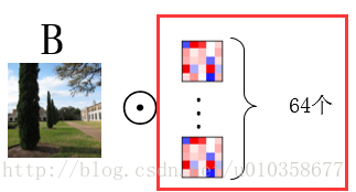
图中用红框圈出的部分即是我们一次展示出的权重参数。
2. 网络权值和feature map的可视化
(1) 网络权重参数可视化
首先介绍一下Tensorflow中卷积核的形状,如下代码所示:
weights = tf.Variable(tf.random_normal([filter_size, filter_size, channels, filter_num]))
- 1
前两维是卷积核的高和宽,第3维是上一层feature map的通道数,在第一节(卷积知识补充)中,我提到了上一层的feature map有多少个(也就是通道数是多少),那么对应着一个卷积核也要有这么多通道。第4维是当前卷积层的卷积核数量,也是当前层输出的feature map的通道数。
以下是我更改之后的网络权重参数(卷积核)的可视化代码:
from __future__ import print_function

#import tensorflow as tf
import numpy as np
import matplotlib.pyplot as plt
import matplotlib.cm as cm
import os
import visualize_utils


def plot_conv_weights(weights, plot_dir, name, channels_all=True, filters_all=True, channels=[0], filters=[0]):
    """
    Plots convolutional filters
    :param weights: numpy array of rank 4
    :param name: string, name of convolutional layer
    :param channels_all: boolean, optional
    :return: nothing, plots are saved on the disk
    """

    w_min = np.min(weights)
    w_max = np.max(weights)

    # make a list of channels if all are plotted
    if channels_all:
        channels = range(weights.shape[2])

    # get number of convolutional filters
    if filters_all:
        num_filters = weights.shape[3]
        filters = range(weights.shape[3])
    else:
        num_filters = len(filters)

    # get number of grid rows and columns
    grid_r, grid_c = visualize_utils.get_grid_dim(num_filters)

    # create figure and axes
    fig, axes = plt.subplots(min([grid_r, grid_c]),
                             max([grid_r, grid_c]))

    # iterate channels
    for channel_ID in channels:
        # iterate filters inside every channel
        if num_filters == 1:
            img = weights[:, :, channel_ID, filters[0]]
            axes.imshow(img, vmin=w_min, vmax=w_max, interpolation='nearest', cmap='seismic')
            # remove any labels from the axes
            axes.set_xticks([])
            axes.set_yticks([])
        else:
            for l, ax in enumerate(axes.flat):
                # get a single filter
                img = weights[:, :, channel_ID, filters[l]]
                # put it on the grid
                ax.imshow(img, vmin=w_min, vmax=w_max, interpolation='nearest', cmap='seismic')
                # remove any labels from the axes
                ax.set_xticks([])
                ax.set_yticks([])
        # save figure
        plt.savefig(os.path.join(plot_dir, '{}-{}.png'.format(name, channel_ID)), bbox_inches='tight')
- 1
- 2
- 3
- 4
- 5
- 6
- 7
- 8
- 9
- 10
- 11
- 12
- 13
- 14
- 15
- 16
- 17
- 18
- 19
- 20
- 21
- 22
- 23
- 24
- 25
- 26
- 27
- 28
- 29
- 30
- 31
- 32
- 33
- 34
- 35
- 36
- 37
- 38
- 39
- 40
- 41
- 42
- 43
- 44
- 45
- 46
- 47
- 48
- 49
- 50
- 51
- 52
- 53
- 54
- 55
- 56
- 57
- 58
- 59
- 60
原项目的代码是对某一层的权重参数或feature map在一个网格中进行全部展示,如果参数或feature map太多,那么展示出来的结果中每个图都很小,很难看出有用的东西来,如下图所示:

所以我对代码做了些修改,使得其能显示任意指定的filter或feature map。
代码中,
w_min = np.min(weights)
w_max = np.max(weights)
- 1
- 2
这两句是为了后续显示图像用的,具体可查看matplotlib.pyplot的imshow()函数进行了解。
接下来是判断是否显示全部的channel(通道数)或全部filter。如果是,那就和原代码一致了。若不是,则画出函数参数channels和filters指定的filter来。
再往下的两句代码是画图用的,我们可能会在一个图中显示多个子图,以下这句是为了计算出大图分为几行几列比较合适(一个大图会尽量分解为方形的阵列,比如如果有64个子图,那么就分成8 x 8的阵列),代码细节可在原项目中的utils中找到。
grid_r, grid_c = visualize_utils.get_grid_dim(num_filters)
- 1
实际画图时,如果想要一个图一个图的去画,需要单独处理一下。如果还是想在一个大图中显示多个子图,就按源代码的方式去做,只不过这里可以显示我们自己指定的那些filter,而不是不加筛选地全部输出。主要拿到数据的是以下这句代码:
img = weights[:, :, channel_ID, filters[l]]
- 1
剩下的都是是画图相关的函数了,本文就不再对画图做更多介绍了。
使用这段代码可视化并保存filter时,先加载模型,然后拿到我们想要可视化的那部分参数,之后直接调用函数就可以了,如下所示:
with tf.Session(graph=tf.get_default_graph()) as sess:
        init_op = tf.group(tf.global_variables_initializer(), tf.local_variables_initializer())
        sess.run(init_op)
        saver.restore(sess, model_path)

        with tf.variable_scope('inference', reuse=True):
            conv_weights = tf.get_variable('conv3_1_w').eval()
            visualize.plot_conv_weights(conv_weights, dir_prefix, 'conv3_1')
- 1
- 2
- 3
- 4
- 5
- 6
- 7
- 8
这里并没有对filter进行额外的指定,在feature map的可视化中,我会给出相关例子。
(2) feature map可视化
其实feature map的可视化与filter非常相似,只有细微的不同。还是先把完整代码贴上。
def plot_conv_output(conv_img, plot_dir, name, filters_all=True, filters=[0]):
    w_min = np.min(conv_img)
    w_max = np.max(conv_img)

    # get number of convolutional filters
    if filters_all:
        num_filters = conv_img.shape[3]
        filters = range(conv_img.shape[3])
    else:
        num_filters = len(filters)

    # get number of grid rows and columns
    grid_r, grid_c = visualize_utils.get_grid_dim(num_filters)

    # create figure and axes
    fig, axes = plt.subplots(min([grid_r, grid_c]),
                             max([grid_r, grid_c]))

    # iterate filters
    if num_filters == 1:
        img = conv_img[0, :, :, filters[0]]
        axes.imshow(img, vmin=w_min, vmax=w_max, interpolation='bicubic', cmap=cm.hot)
        # remove any labels from the axes
        axes.set_xticks([])
        axes.set_yticks([])
    else:
        for l, ax in enumerate(axes.flat):
            # get a single image
            img = conv_img[0, :, :, filters[l]]
            # put it on the grid
            ax.imshow(img, vmin=w_min, vmax=w_max, interpolation='bicubic', cmap=cm.hot)
            # remove any labels from the axes
            ax.set_xticks([])
            ax.set_yticks([])
    # save figure
    plt.savefig(os.path.join(plot_dir, '{}.png'.format(name)), bbox_inches='tight')
- 1
- 2
- 3
- 4
- 5
- 6
- 7
- 8
- 9
- 10
- 11
- 12
- 13
- 14
- 15
- 16
- 17
- 18
- 19
- 20
- 21
- 22
- 23
- 24
- 25
- 26
- 27
- 28
- 29
- 30
- 31
- 32
- 33
- 34
- 35
- 36
代码中和filter可视化相同的部分就不再赘述了,这里只讲feature map可视化独特的方面,其实就在于以下这句代码,也就是要可视化的数据的获得:
img = conv_img[0, :, :, filters[0]]
- 1
神经网络一般都是一个batch一个batch的输入数据,其输入的形状为
image = tf.placeholder(tf.float32, shape = [None, IMAGE_SIZE, IMAGE_SIZE, 3], name = "input_image")
- 1
第一维是一个batch中图片的数量,为了灵活可以设置为None,Tensorflow会根据实际输入的数据进行计算。二三维是图片的高和宽,第4维是图片通道数,一般为3。
如果我们想要输入一幅图片,然后看看它的激活值(feature map),那么也要按照以上维度以一个batch的形式进行输入,也就是[1, IMAGE_SIZE, IMAGE_SIZE, 3]。所以拿feature map数据时,第一维度肯定是取0(就对应着batch中的当前图片),二三维取全部,第4维度再取我们想要查看的feature map的某一通道。
如果想要可视化feature map,那么构建网络时还要动点手脚,定义计算图时,每得到一组激活值都要将其加到Tensorflow的collection中,如下:
tf.add_to_collection('activations', current)
- 1
而实际进行feature map可视化时,就要先输入一幅图片,然后运行网络拿到相应数据,最后把数据传参给可视化函数。以下这个例子展示的是如何将每个指定卷积层的feature map的每个通道进行单独的可视化与存储,使用的是VGG16网络:
visualize_layers = ['conv1_1', 'conv1_2', 'conv2_1', 'conv2_2', 'conv3_1', 'conv3_2', 'conv3_3', 'conv4_1', 'conv4_2', 'conv4_3', 'conv5_1', 'conv5_2', 'conv5_3']

with tf.Session(graph=tf.get_default_graph()) as sess:
        init_op = tf.group(tf.global_variables_initializer(), tf.local_variables_initializer())
        sess.run(init_op)
        saver.restore(sess, model_path)

        image_path = root_path + 'images/train_images/sunny_0058.jpg'
        img = misc.imread(image_path)
        img = img - meanvalue
        img = np.float32(img)
        img = np.expand_dims(img, axis=0)

        conv_out = sess.run(tf.get_collection('activations'), feed_dict={x: img, keep_prob: 1.0})
        for i, layer in enumerate(visualize_layers):
            visualize_utils.create_dir(dir_prefix + layer)
            for j in range(conv_out[i].shape[3]):
                visualize.plot_conv_output(conv_out[i], dir_prefix + layer, str(j), filters_all=False, filters=[j])

        sess.close()
- 1
- 2
- 3
- 4
- 5
- 6
- 7
- 8
- 9
- 10
- 11
- 12
- 13
- 14
- 15
- 16
- 17
- 18
- 19
- 20
其中,conv_out包含了所有加入到collection中的feature map,这些feature map在conv_out中是按卷积层划分的。
最终得到的结果如下图所示:

第一个文件夹下的全部结果:

                                        <div class="markdown_views">
            <h2 id="前言"><a name="t0"></a>前言</h2>
Tensorflow中可以使用tensorboard这个强大的工具对计算图、loss、网络参数等进行可视化。本文并不涉及对tensorboard使用的介绍,而是旨在说明如何通过代码对网络权值和feature map做更灵活的处理、显示和存储。本文的相关代码主要参考了github上的一个小项目,但是对其进行了改进。原项目地址为(https://github.com/grishasergei/conviz)。
本文将从以下两个方面进行介绍:
- 卷积知识补充
- 网络权值和feature map的可视化
1. 卷积知识补充
为了后面方便讲解代码,这里先对卷积的部分知识进行一下简介。关于卷积核如何在图像的一个通道上进行滑动计算,网上有诸多资料,相信对卷积神经网络有一定了解的读者都应该比较清楚,本文就不再赘述。这里主要介绍一组卷积核如何在一幅图像上计算得到一组feature map。
以从原始图像经过第一个卷积层得到第一组feature map为例(从得到的feature map到再之后的feature map也是同理),假设第一组feature map共有64个,那么可以把这组feature map也看作一幅图像,只不过它的通道数是64, 而一般意义上的图像是RGB3个通道。为了得到这第一组feature map,我们需要64个卷积核,每个卷积核是一个k x k x 3的矩阵,其中k是卷积核的大小(假设是正方形卷积核),3就对应着输入图像的通道数。下面我以一个简单粗糙的图示来展示一下图像经过一个卷积核的卷积得到一个feature map的过程。
如图所示,其实可以看做卷积核的每一通道(不太准确,将就一下)和图像的每一通道对应进行卷积操作,然后再逐位置相加,便得到了一个feature map。
那么用一组(64个)卷积核去卷积一幅图像,得到64个feature map就如下图所示,也就是每个卷积核得到一个feature map,64个卷积核就得到64个feature map。
另外,也可以稍微换一个角度看待这个问题,那就是先让图片的某一通道分别与64个卷积核的对应通道做卷积,得到64个feature map的中间结果,之后3个通道对应的中间结果再相加,得到最终的feature map,如下图所示:
可以看到这其实就是第一幅图扩展到多卷积核的情形,图画得较为粗糙,有些中间结果和最终结果直接用了一样的子图,理解时请稍微注意一下。下面代码中对卷积核进行展示的时候使用的就是这种方式,即对应着输入图像逐通道的去显示卷积核的对应通道,而不是每次显示一个卷积核的所有通道,可能解释的有点绕,需要注意一下。通过下面这个小图也许更好理解。
图中用红框圈出的部分即是我们一次展示出的权重参数。
2. 网络权值和feature map的可视化
(1) 网络权重参数可视化
首先介绍一下Tensorflow中卷积核的形状,如下代码所示:
weights = tf.Variable(tf.random_normal([filter_size, filter_size, channels, filter_num]))
- 1
前两维是卷积核的高和宽,第3维是上一层feature map的通道数,在第一节(卷积知识补充)中,我提到了上一层的feature map有多少个(也就是通道数是多少),那么对应着一个卷积核也要有这么多通道。第4维是当前卷积层的卷积核数量,也是当前层输出的feature map的通道数。
以下是我更改之后的网络权重参数(卷积核)的可视化代码:
from __future__ import print_function

#import tensorflow as tf
import numpy as np
import matplotlib.pyplot as plt
import matplotlib.cm as cm
import os
import visualize_utils


def plot_conv_weights(weights, plot_dir, name, channels_all=True, filters_all=True, channels=[0], filters=[0]):
    """
    Plots convolutional filters
    :param weights: numpy array of rank 4
    :param name: string, name of convolutional layer
    :param channels_all: boolean, optional
    :return: nothing, plots are saved on the disk
    """

    w_min = np.min(weights)
    w_max = np.max(weights)

    # make a list of channels if all are plotted
    if channels_all:
        channels = range(weights.shape[2])

    # get number of convolutional filters
    if filters_all:
        num_filters = weights.shape[3]
        filters = range(weights.shape[3])
    else:
        num_filters = len(filters)

    # get number of grid rows and columns
    grid_r, grid_c = visualize_utils.get_grid_dim(num_filters)

    # create figure and axes
    fig, axes = plt.subplots(min([grid_r, grid_c]),
                             max([grid_r, grid_c]))

    # iterate channels
    for channel_ID in channels:
        # iterate filters inside every channel
        if num_filters == 1:
            img = weights[:, :, channel_ID, filters[0]]
            axes.imshow(img, vmin=w_min, vmax=w_max, interpolation='nearest', cmap='seismic')
            # remove any labels from the axes
            axes.set_xticks([])
            axes.set_yticks([])
        else:
            for l, ax in enumerate(axes.flat):
                # get a single filter
                img = weights[:, :, channel_ID, filters[l]]
                # put it on the grid
                ax.imshow(img, vmin=w_min, vmax=w_max, interpolation='nearest', cmap='seismic')
                # remove any labels from the axes
                ax.set_xticks([])
                ax.set_yticks([])
        # save figure
        plt.savefig(os.path.join(plot_dir, '{}-{}.png'.format(name, channel_ID)), bbox_inches='tight')
- 1
- 2
- 3
- 4
- 5
- 6
- 7
- 8
- 9
- 10
- 11
- 12
- 13
- 14
- 15
- 16
- 17
- 18
- 19
- 20
- 21
- 22
- 23
- 24
- 25
- 26
- 27
- 28
- 29
- 30
- 31
- 32
- 33
- 34
- 35
- 36
- 37
- 38
- 39
- 40
- 41
- 42
- 43
- 44
- 45
- 46
- 47
- 48
- 49
- 50
- 51
- 52
- 53
- 54
- 55
- 56
- 57
- 58
- 59
- 60
原项目的代码是对某一层的权重参数或feature map在一个网格中进行全部展示,如果参数或feature map太多,那么展示出来的结果中每个图都很小,很难看出有用的东西来,如下图所示:
所以我对代码做了些修改,使得其能显示任意指定的filter或feature map。
代码中,
w_min = np.min(weights)
w_max = np.max(weights)
- 1
- 2
这两句是为了后续显示图像用的,具体可查看matplotlib.pyplot的imshow()函数进行了解。
接下来是判断是否显示全部的channel(通道数)或全部filter。如果是,那就和原代码一致了。若不是,则画出函数参数channels和filters指定的filter来。
再往下的两句代码是画图用的,我们可能会在一个图中显示多个子图,以下这句是为了计算出大图分为几行几列比较合适(一个大图会尽量分解为方形的阵列,比如如果有64个子图,那么就分成8 x 8的阵列),代码细节可在原项目中的utils中找到。
grid_r, grid_c = visualize_utils.get_grid_dim(num_filters)
- 1
实际画图时,如果想要一个图一个图的去画,需要单独处理一下。如果还是想在一个大图中显示多个子图,就按源代码的方式去做,只不过这里可以显示我们自己指定的那些filter,而不是不加筛选地全部输出。主要拿到数据的是以下这句代码:
img = weights[:, :, channel_ID, filters[l]]
- 1
剩下的都是是画图相关的函数了,本文就不再对画图做更多介绍了。
使用这段代码可视化并保存filter时,先加载模型,然后拿到我们想要可视化的那部分参数,之后直接调用函数就可以了,如下所示:
with tf.Session(graph=tf.get_default_graph()) as sess:
        init_op = tf.group(tf.global_variables_initializer(), tf.local_variables_initializer())
        sess.run(init_op)
        saver.restore(sess, model_path)

        with tf.variable_scope('inference', reuse=True):
            conv_weights = tf.get_variable('conv3_1_w').eval()
            visualize.plot_conv_weights(conv_weights, dir_prefix, 'conv3_1')
- 1
- 2
- 3
- 4
- 5
- 6
- 7
- 8
这里并没有对filter进行额外的指定,在feature map的可视化中,我会给出相关例子。
(2) feature map可视化
其实feature map的可视化与filter非常相似,只有细微的不同。还是先把完整代码贴上。
def plot_conv_output(conv_img, plot_dir, name, filters_all=True, filters=[0]):
    w_min = np.min(conv_img)
    w_max = np.max(conv_img)

    # get number of convolutional filters
    if filters_all:
        num_filters = conv_img.shape[3]
        filters = range(conv_img.shape[3])
    else:
        num_filters = len(filters)

    # get number of grid rows and columns
    grid_r, grid_c = visualize_utils.get_grid_dim(num_filters)

    # create figure and axes
    fig, axes = plt.subplots(min([grid_r, grid_c]),
                             max([grid_r, grid_c]))

    # iterate filters
    if num_filters == 1:
        img = conv_img[0, :, :, filters[0]]
        axes.imshow(img, vmin=w_min, vmax=w_max, interpolation='bicubic', cmap=cm.hot)
        # remove any labels from the axes
        axes.set_xticks([])
        axes.set_yticks([])
    else:
        for l, ax in enumerate(axes.flat):
            # get a single image
            img = conv_img[0, :, :, filters[l]]
            # put it on the grid
            ax.imshow(img, vmin=w_min, vmax=w_max, interpolation='bicubic', cmap=cm.hot)
            # remove any labels from the axes
            ax.set_xticks([])
            ax.set_yticks([])
    # save figure
    plt.savefig(os.path.join(plot_dir, '{}.png'.format(name)), bbox_inches='tight')
- 1
- 2
- 3
- 4
- 5
- 6
- 7
- 8
- 9
- 10
- 11
- 12
- 13
- 14
- 15
- 16
- 17
- 18
- 19
- 20
- 21
- 22
- 23
- 24
- 25
- 26
- 27
- 28
- 29
- 30
- 31
- 32
- 33
- 34
- 35
- 36
代码中和filter可视化相同的部分就不再赘述了,这里只讲feature map可视化独特的方面,其实就在于以下这句代码,也就是要可视化的数据的获得:
img = conv_img[0, :, :, filters[0]]
- 1
神经网络一般都是一个batch一个batch的输入数据,其输入的形状为
image = tf.placeholder(tf.float32, shape = [None, IMAGE_SIZE, IMAGE_SIZE, 3], name = "input_image")
- 1
第一维是一个batch中图片的数量,为了灵活可以设置为None,Tensorflow会根据实际输入的数据进行计算。二三维是图片的高和宽,第4维是图片通道数,一般为3。
如果我们想要输入一幅图片,然后看看它的激活值(feature map),那么也要按照以上维度以一个batch的形式进行输入,也就是[1, IMAGE_SIZE, IMAGE_SIZE, 3]。所以拿feature map数据时,第一维度肯定是取0(就对应着batch中的当前图片),二三维取全部,第4维度再取我们想要查看的feature map的某一通道。
如果想要可视化feature map,那么构建网络时还要动点手脚,定义计算图时,每得到一组激活值都要将其加到Tensorflow的collection中,如下:
tf.add_to_collection('activations', current)
- 1
而实际进行feature map可视化时,就要先输入一幅图片,然后运行网络拿到相应数据,最后把数据传参给可视化函数。以下这个例子展示的是如何将每个指定卷积层的feature map的每个通道进行单独的可视化与存储,使用的是VGG16网络:
visualize_layers = ['conv1_1', 'conv1_2', 'conv2_1', 'conv2_2', 'conv3_1', 'conv3_2', 'conv3_3', 'conv4_1', 'conv4_2', 'conv4_3', 'conv5_1', 'conv5_2', 'conv5_3']

with tf.Session(graph=tf.get_default_graph()) as sess:
        init_op = tf.group(tf.global_variables_initializer(), tf.local_variables_initializer())
        sess.run(init_op)
        saver.restore(sess, model_path)

        image_path = root_path + 'images/train_images/sunny_0058.jpg'
        img = misc.imread(image_path)
        img = img - meanvalue
        img = np.float32(img)
        img = np.expand_dims(img, axis=0)

        conv_out = sess.run(tf.get_collection('activations'), feed_dict={x: img, keep_prob: 1.0})
        for i, layer in enumerate(visualize_layers):
            visualize_utils.create_dir(dir_prefix + layer)
            for j in range(conv_out[i].shape[3]):
                visualize.plot_conv_output(conv_out[i], dir_prefix + layer, str(j), filters_all=False, filters=[j])

        sess.close()
- 1
- 2
- 3
- 4
- 5
- 6
- 7
- 8
- 9
- 10
- 11
- 12
- 13
- 14
- 15
- 16
- 17
- 18
- 19
- 20
其中,conv_out包含了所有加入到collection中的feature map,这些feature map在conv_out中是按卷积层划分的。
最终得到的结果如下图所示:
第一个文件夹下的全部结果: