案例一
matlab代码:
clc,clear;
x=[5 10 20 30 40 50 60 70 80 90]
x =
5 10 20 30 40 50 60 70 80 90
>> y=[0 19 57 94 134 173 216 256 297 343]
y =
0 19 57 94 134 173 216 256 297 343
>> R=[5 10 20 30 40 50 60 70 80 90]'
R =
5
10
20
30
40
50
60
70
80
90
>> Y=[0 19 57 94 134 173 216 256 297 343]'
Y =
0
19
57
94
134
173
216
256
297
343
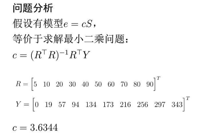
>> c=inv(R'*R)*R'*Y
c =
3.6344
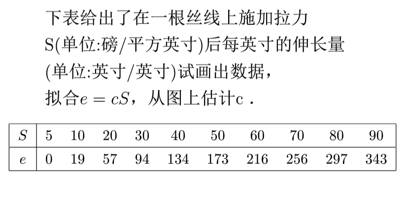
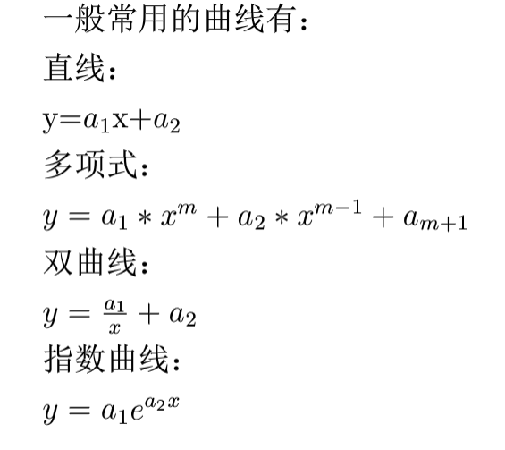
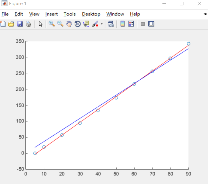
如果题目没有给出拟合的模型,通常我们将数据做成散点图,直观的去判断应该用什么样的曲线去拟合。
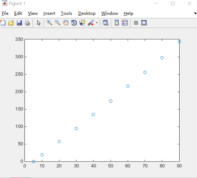
我们先画出这个问题的散点图
plot(x,y,'o')
然后对数据做线性拟合:(接着上面代码输入)
hold on
>> p=polyfit(x,y,1)
p =
4.0103 -23.5682
>> y1=4.0103.*x-23.5682
y1 =
Columns 1 through 6
-3.5167 16.5348 56.6378 96.7408 136.8438 176.9468
Columns 7 through 10
217.0498 257.1528 297.2558 337.3588
>> y=3.6344.*x
y =
Columns 1 through 6
18.1720 36.3440 72.6880 109.0320 145.3760 181.7200
Columns 7 through 10
218.0640 254.4080 290.7520 327.0960
>> plot(x,y1,'r',x,y,'b')
运行结果
案例二
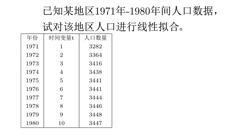
依旧是用matlab画出数据的散点图,代码如下:
clc,clear;
x=[1:1:10]
x =
1 2 3 4 5 6 7 8 9 10
>> y=[3282 3364 3416 3438 3441 3441 3444 3446 3448 3447]
y =
Columns 1 through 5
3282 3364 3416 3438 3441
Columns 6 through 10
3441 3444 3446 3448 3447
>> xlabel('time')
>> ylabel('population')
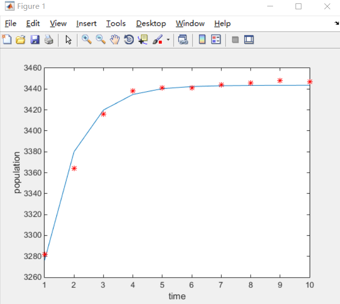
>> plot(x,y,'r*')
运行结果:
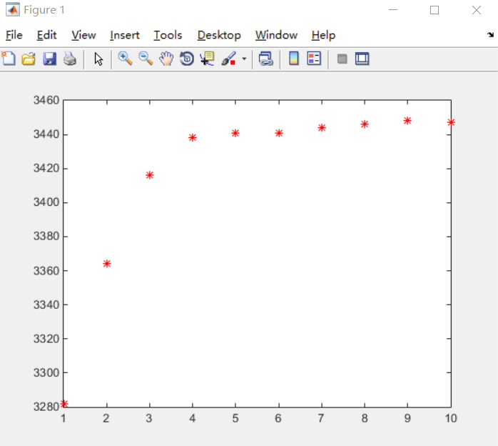
分析:从图中我们可以看出人口随时间变化是个非线性过程,考虑到散点图形状以及人口模型一般涉及Logistic曲线模型,所以我们这个用这个模型,基本形式为
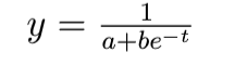
我们要经过数据变化变成一个线性模型,取x'=e^-x,y'=1/y,则原模型可转换为线性模型y'=a+bx',然后使用matlab进行拟合,代码如下:
x0=exp(-x)
x0 =
Columns 1 through 6
0.3679 0.1353 0.0498 0.0183 0.0067 0.0025
Columns 7 through 10
0.0009 0.0003 0.0001 0.0000
>> y0=1./y
y0 =
1.0e-03 *
Columns 1 through 6
0.3047 0.2973 0.2927 0.2909 0.2906 0.2906
Columns 7 through 10
0.2904 0.2902 0.2900 0.2901
>> f=polyfit(x0,y0,1)
f =
1.0e-03 *
0.0403 0.2904
>> y_fit=1./(f(1).*exp(-x)+f(2))
y_fit =
1.0e+03 *
Columns 1 through 6
3.2761 3.3800 3.4199 3.4348 3.4403 3.4423
Columns 7 through 10
3.4431 3.4434 3.4435 3.4435
>> plot(x,y_fit)
>> hold on
>> xlabel('time')
>> ylabel('population')
>> plot(x,y,'r*')
运行结果:
所以我们最终得到的拟合曲线为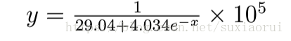
关于这类问题先画出散点图然后观察是什么模型,然后进行拟合。最终带到拟合曲线,和原数据进行比对,看是否符合。