做线性回归模型,1、增加多项式特征可以克服欠拟合问题,提高模型的效果,2、对特征进行归一化虽然无法提高预测精度,当可以提高计算效率。
from sklearn.linear_model  import LinearRegression
from sklearn.preprocessing import PolynomialFeatures
from sklearn.pipeline import Pipeline
import numpy as np
import matplotlib.pyplot as plt

def polynomial_model(degree = 1):
    polynomial_features = PolynomialFeatures(degree = degree, include_bias = False)
    ## degree > 1 可以构造增加多项式特征
    linear_regression = LinearRegression(normalize = True)
    ## 对特征进行归一化
    pipeline = Pipeline([('polynomial_features', polynomial_features), ('linear_regression', linear_regression)])
    return pipeline
n_dots = 200
X = np.linspace(-2*np.pi, 2*np.pi, n_dots)
Y = np.sin(X) + 0.1*np.random.randn(n_dots) - 0.1
X = X.reshape(-1, 1)
## X为-2pi到2pi上的等间距的数组
Y = Y.reshape(-1, 1)
## Y为X对应的正弦值加一定的噪声得到的
from sklearn.metrics import mean_squared_error
## mean_squared_error为样本均方误差函数
degrees = [2, 3, 5, 10]
results = []
for d in degrees:
model = polynomial_model(degree = d)
model.fit(X, Y)
train_score = model.score(X, Y) ## 这里的score为拟合优度
mse = mean_squared_error(Y, model.predict(X))
## mean_squared_error为样本均方误差函数
results.append({"model": model, "degree": d, "score": train_score, "mse": mse})
for r in results:
print("degree: {}; train score: {}; mean squared error: {}".format(r["degree"], r["score"], r["mse"]))mean_squared_error(Y, Y_hat)为样本均方误差函数:
运行结果:
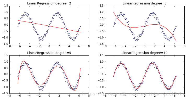
degree: 2;   train score: 0.1445946099267632;   mean squared error: 0.431381922441344
degree: 3;   train score: 0.275972368454415;   mean squared error: 0.3651279676529122
degree: 5;   train score: 0.8972167262379881;   mean squared error: 0.05183372322037336
degree: 10;   train score: 0.9821185979705528;   mean squared error: 0.009017611617748928
可以看出degree为10时,拟合优度最高,MSE最小。
from matplotlib.figure import SubplotParams

plt.figure(figsize = (12, 6), dpi = 200, subplotpars = SubplotParams(hspace = 0.3))
for i, r in enumerate(results):
    fig = plt.subplot(2, 2, i + 1)
    plt.xlim(-8, 8)
    plt.title("LinearRegression degree={}".format(r["degree"]))
    plt.scatter(X, Y, s = 5, c = 'b', alpha = 0.5)
    plt.plot(X, r["model"].predict(X), 'r-')
运行结果: