1. 抓取影评
一般影评网站都有反爬虫机制,而且每个网站的都不尽相同,所以需要采取一些手段并根据具体网站的情况来进行爬取,本文以my为例
df = pd.DataFrame(columns=['date', 'score', 'city', 'comment', 'nick'])
for i in range(1000):
    j = random.randint(1, 1000)
    print(str(i) + 'th '+'download page: ' + str(j))
    try:
        time.sleep(2)
        url = 'http://m.maoyan.com/mmdb/comments/movie/1216446.json?_v_=yes&offset=' + str(j)
        html = requests.get(url=url).content
        data = json.loads(html.decode('utf-8'))['cmts']
        for item in data:
            df = df.append({'date': item['time'].split(' ')[0],
                          'city': item['cityName'],
                          'score': item['score'],
                          'comment': item['content'],
                          'nick': item['nick']}, ignore_index=True)
        with open('./filmreview/take-my-bro3.csv', 'a+', encoding='utf-8') as fhand:
            df.to_csv(fhand, index=False)
    except Exception as e:
        print('Error processed: %s' % e)
continue- 找到特定电影的评论在其移动门户中的url,然后按页面爬取且随机生成页码
- 每休眠2s后再进行爬取,以免过于频繁
- 还有就是需要注意将网络数据写入本地时需指明编码方式为utf-8否则会出现编码错误的问题
2. 可视化分析
首先加载先前写入本地的数据,并进行适当处理
# load data
data_path = './filmreview/take-my-bro3.csv'
df = pd.read_csv(data_path)

# convert the  str socre into float
score_list = []
for s in df['score']:
    if s == 'score':
        s = 0
    score_list.append(float(s))

new_score = {'score_float': score_list}
new_score = pd.DataFrame(new_score)
df = pd.concat([df, new_score], axis=1)
# count the number of comment and average score
grouped = df.groupby(['city'])
grouped_pct = grouped['score_float']
city_com = grouped_pct.agg(['mean', 'count'])
city_com.reset_index(inplace=True)
data = [(city_com['city'][i], city_com['count'][i]) for i in range(0, city_com.shape[0])]- 因为载入文件的分数项类型为字符,所以需要先转换为浮点型数值才能进行接下来的分组聚合操作
- 然后将数据表按城市项进行分组,即同一城市的分为一组。再对按组分的数据提取评分项计算个数以及平均值,最后拿出城市和对应的评论数
2.1 绘制全国热力图
使用百度提供的开源js可视化库pyecharts,需要预先进行安装(直接命令行 pip install pyecharts),但需要注意的是由于官方处于轻量级的考虑已经不再内置地图包,所以还需要进行额外安装,具体操作请看
from pyecharts import Geo
geo = Geo('Take my bro. away national heatmap', title_color="#fff", title_pos="center", width=1200, height=600, background_color='#404a59')
attr, value = geo.cast(data)
geo.add("", attr, value, type="heatmap", visual_range=[0, 200],visual_text_color="#fff", symbol_size=10, is_visualmap=True,is_roam=False)
geo.render("./filmreview/test.html")- 但需要注意的是,有些较小的城市地图包里也没有,此时只有两种解决方案:
1 手动添加城市及其经纬度
geo.add_coordinate('万宁', 18.47, 110.23)2 获取已下载地图包含的城市列表并删除不支持的城市
import json
with open('./filmreview/city_coordinates.json', 'r', encoding='utf-8') as fhand:
    city = json.load(fhand)
for i in range(len(attr)):
    if attr[i] not in city:
        del attr[i]
del value[i] - 因为安装地图包时已下载好该文件,所以直接本地查找到然后复制到工作目录
- 又较小城市多(大概70个)且对分析的影响不大,所以本例采用直接删除的方式
- 还需要注意中文编码问题,因为python2内置编码方式是unicode,即不同编码格式的转换都是以unicode为中介进行转换的,而出现编码错误一般解决方案是重置默认编码方式为utf-8。如果不可行建议更换版本为python3,因为3的编码兼容性比2要好得多(笑)
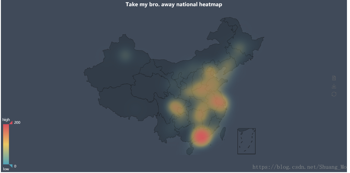
- 此外就是,当爬取的数据较多时,数据值差距较大,会出现颜色覆盖的问题(如下图),则就需要对数值进行归一化处理再根据实际颜色情况适当放大
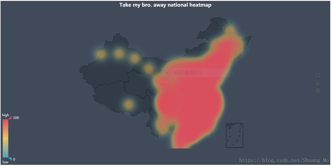
value /= (max(value) - min(value))
value *= 200
最终绘出全国热力图如下
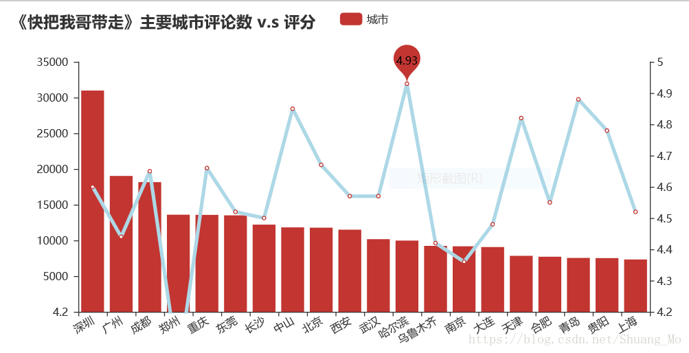
2.2 绘制折线图与柱状图
from pyecharts import Line, Bar, Overlap
city_main = city_com.sort_values('count', ascending=False)[0:20]
attr = city_main['city']
v1 = city_main['count']

S = []
scores = city_main['mean']
for s in scores:
    S.append(round(s, 2))
v2 = S

line = Line("主要城市评价")

line.add("城市", attr, v2, is_stack=True, xaxis_rotate=30, yaxis_min=4.2,
        mark_point=['min',  'max'], xaxis_interval=0, line_color='lightblue',
        line_width=4, mark_point_textcolor='black', mark_point_color='light_blue',
        is_splitline_show=False)
bar = Bar("《快把我哥带走》主要城市评论数 v.s 评分")

bar.add("城市", attr, v1, is_stack=True, xaxis_rotate=30, yaxis_min=4.2,
       xaxis_interval=0, is_splitline_show=False)

overlap = Overlap()

# default not add new x, y axis and the index of x, y both are 0
overlap.add(bar)

overlap.add(line, yaxis_index=1, is_add_yaxis=True)
overlap.render('./filmreview/line_test.html')
绘出图形如下
2.3 词云图
制作词云图需要安装第三方库wordcloud和jieba(进行中文分词)
首先将评论文本提取出来并进行分词
word_str = ' '.join(df['comment'])
word_list = []
word_generator = jieba.cut_for_search(word_str)
for word in word_generator:
    word_list.append(word)
words_list = [k for k in word_list if len(k) > 1]
然后选择素材图片(要求清晰、色彩鲜明且背景色为白色(本例))来制作词云图,再统计字词的出现频率最后完成词云图
back_color = imread('./filmreview/mybro2.jpg') # parse the image
wc = WordCloud(background_color='white',
              max_words=200,
              mask=back_color,
              max_font_size=300,
              stopwords=STOPWORDS.add('苟利国'),
              font_path='C:/Windows/Fonts/SIMYOU.TTF',
              random_state=42)
word_count = Counter(words_list)
wc.generate_from_frequencies(word_count)
image_colors = ImageColorGenerator(back_color)
fig = plt.figure()
ax = fig.add_subplot(1, 1, 1)
ax.imshow(wc.recolor(color_func=image_colors))
ax.set_title("WordCloud of  'Take my bro. away'. by:Mosan" )
ax.axis('off')- 若最后效果满意可使用plt.savefig()写入本地
素材图和效果图如下:


扫描二维码关注公众号,回复:
2904333 查看本文章

End.
参考教程:
1. 3天破9亿!上万条评论解读《西虹市首富》是否值得一看
2. Python 005- 使用Pyecharts来绘制各种各样的图形
相关链接:
影评数据集