1 - Task
- Implement the neural style transfer algorithm
- Generate novel artistic images using your algorithm
2 - Import Packages
import os
import sys
import scipy.io
import scipy.misc
import matplotlib.pyplot as plt
from matplotlib.pyplot import imshow
from PIL import Image
from nst_utils import *
import numpy as np
import tensorflow as tf

%matplotlib inline
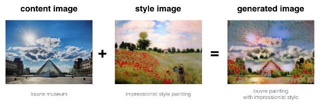
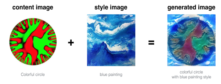
3 - Problem Statement
4 - Transfer Learning
加载已经在ImageNet数据集上训练好的VGG网络。
model = load_vgg_model("pretrained-model/imagenet-vgg-verydeep-19.mat")
print(model)
Result:
{'conv5_3': <tf.Tensor 'Relu_14:0' shape=(1, 19, 25, 512) dtype=float32>, 'avgpool1': <tf.Tensor 'AvgPool:0' shape=(1, 150, 200, 64) dtype=float32>, 'conv5_2': <tf.Tensor 'Relu_13:0' shape=(1, 19, 25, 512) dtype=float32>, 'conv3_3': <tf.Tensor 'Relu_6:0' shape=(1, 75, 100, 256) dtype=float32>, 'conv3_2': <tf.Tensor 'Relu_5:0' shape=(1, 75, 100, 256) dtype=float32>, 'conv4_2': <tf.Tensor 'Relu_9:0' shape=(1, 38, 50, 512) dtype=float32>, 'avgpool3': <tf.Tensor 'AvgPool_2:0' shape=(1, 38, 50, 256) dtype=float32>, 'conv4_3': <tf.Tensor 'Relu_10:0' shape=(1, 38, 50, 512) dtype=float32>, 'avgpool5': <tf.Tensor 'AvgPool_4:0' shape=(1, 10, 13, 512) dtype=float32>, 'conv3_1': <tf.Tensor 'Relu_4:0' shape=(1, 75, 100, 256) dtype=float32>, 'conv5_1': <tf.Tensor 'Relu_12:0' shape=(1, 19, 25, 512) dtype=float32>, 'conv2_2': <tf.Tensor 'Relu_3:0' shape=(1, 150, 200, 128) dtype=float32>, 'conv5_4': <tf.Tensor 'Relu_15:0' shape=(1, 19, 25, 512) dtype=float32>, 'input': <tf.Variable 'Variable:0' shape=(1, 300, 400, 3) dtype=float32_ref>, 'conv3_4': <tf.Tensor 'Relu_7:0' shape=(1, 75, 100, 256) dtype=float32>, 'conv4_1': <tf.Tensor 'Relu_8:0' shape=(1, 38, 50, 512) dtype=float32>, 'conv4_4': <tf.Tensor 'Relu_11:0' shape=(1, 38, 50, 512) dtype=float32>, 'avgpool2': <tf.Tensor 'AvgPool_1:0' shape=(1, 75, 100, 128) dtype=float32>, 'avgpool4': <tf.Tensor 'AvgPool_3:0' shape=(1, 19, 25, 512) dtype=float32>, 'conv1_1': <tf.Tensor 'Relu:0' shape=(1, 300, 400, 64) dtype=float32>, 'conv2_1': <tf.Tensor 'Relu_2:0' shape=(1, 150, 200, 128) dtype=float32>, 'conv1_2': <tf.Tensor 'Relu_1:0' shape=(1, 300, 400, 64) dtype=float32>}
5 - Neural Style Transfer
实现NST算法有如下几个步骤:
- Build the content cost function Jcontent(C,G)Jcontent(C,G)
- Build the style cost function Jstyle(S,G)Jstyle(S,G)
- Put it together to get J(G)=αJcontent(C,G)+βJstyle(S,G)J(G)=αJcontent(C,G)+βJstyle(S,G).
5.1 - Computing the content cost
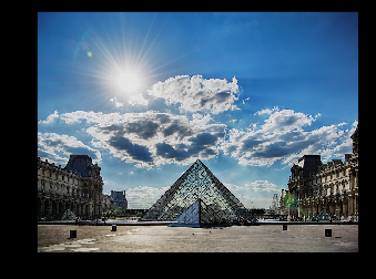
浏览浏览图片。
content_image = scipy.misc.imread("images/louvre.jpg")
imshow(content_image)
Result:
<matplotlib.image.AxesImage at 0x21eca6026d8>
5.1.1 - How do you ensure the generated image G matches the content of the image C?
内容损失函数如下:
$$J_{content}(C,G) = \frac{1}{4 \times n_H \times n_W \times n_C}\sum _{ \text{all entries}} (a^{(C)} - a^{(G)})^2\tag{1} $$
实现$compute_content_cost()$方法有如下步骤:
- Retrieve dimensions from a_G:
- To retrieve dimensions from a tensor X, use:
X.get_shape().as_list()
- To retrieve dimensions from a tensor X, use:
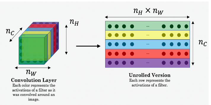
- Unroll a_C and a_G as explained in the picture above
- Compute the content cost:
# GRADED FUNCTION: compute_content_cost

def compute_content_cost(a_C, a_G):
    """
    Computes the content cost

    Arguments:
    a_C -- tensor of dimension (1, n_H, n_W, n_C), hidden layer activations representing content of the image C
    a_G -- tensor of dimension (1, n_H, n_W, n_C), hidden layer activations representing content of the image G

    Returns:
    J_content -- scalar that you compute using equation 1 above.
    """

    ### START CODE HERE ###
    # Retrieve dimensions from a_G (≈1 line)
    m, n_H, n_W, n_C = a_G.get_shape().as_list()

    # Reshape a_C and a_G (≈2 lines)
    a_C_unrolled = tf.reshape(a_C, (n_H*n_W, n_C))
    a_G_unrolled = tf.reshape(a_G, (n_H*n_W, n_C))# compute the cost with tensorflow (≈1 line)
    J_content = 1 / (4*n_H*n_W*n_C) * tf.reduce_sum(tf.square(tf.subtract(a_C_unrolled, a_G_unrolled)))
    ### END CODE HERE ###

    return J_content
tf.reset_default_graph()

with tf.Session() as test:
    tf.set_random_seed(1)
    a_C = tf.random_normal([1, 4, 4, 3], mean=1, stddev=4)
    a_G = tf.random_normal([1, 4, 4, 3], mean=1, stddev=4)
    J_content = compute_content_cost(a_C, a_G)
    print("J_content = " + str(J_content.eval()))
Result:
J_content = 6.76559
5.2 - Computing the style cost
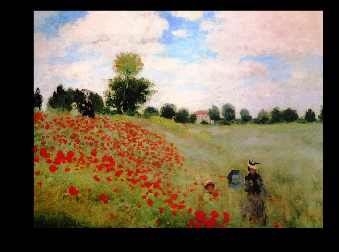
预览图片。
style_image = scipy.misc.imread("images/monet_800600.jpg")
imshow(style_image)
Result:
<matplotlib.image.AxesImage at 0x21eccaeff28>
5.2.1 - Style matrix
$$G_A = AA^T$$
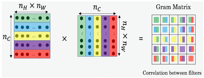
# GRADED FUNCTION: gram_matrix

def gram_matrix(A):
    """
    Argument:
    A -- matrix of shape (n_C, n_H*n_W)

    Returns:
    GA -- Gram matrix of A, of shape (n_C, n_C)
    """

    ### START CODE HERE ### (≈1 line)
    GA = tf.matmul(A, tf.transpose(A))
    ### END CODE HERE ###

    return GA
tf.reset_default_graph()

with tf.Session() as test:
    tf.set_random_seed(1)
    A = tf.random_normal([3, 2*1], mean=1, stddev=4)
    GA = gram_matrix(A)

    print("GA = " + str(GA.eval()))
Result:
GA = [[  6.42230511  -4.42912197  -2.09668207]
 [ -4.42912197  19.46583748  19.56387138]
 [ -2.09668207  19.56387138  20.6864624 ]]
5.2.2 - Style cost
风格损失函数如下:
$$J_{style}^{[l]}(S,G) = \frac{1}{4 \times {n_C}^2 \times (n_H \times n_W)^2} \sum _{i=1}^{n_C}\sum_{j=1}^{n_C}(G^{(S)}_{ij} - G^{(G)}_{ij})^2\tag{2} $$
实现$compute_layer_style_cost()$方法有如下步骤:
- Retrieve dimensions from the hidden layer activations a_G:
- To retrieve dimensions from a tensor X, use:
X.get_shape().as_list()
- To retrieve dimensions from a tensor X, use:
- Unroll the hidden layer activations a_S and a_G into 2D matrices, as explained in the picture above.
- Compute the Style matrix of the images S and G. (Use the function you had previously written.)
- Compute the Style cost:
# GRADED FUNCTION: compute_layer_style_cost

def compute_layer_style_cost(a_S, a_G):
    """
    Arguments:
    a_S -- tensor of dimension (1, n_H, n_W, n_C), hidden layer activations representing style of the image S
    a_G -- tensor of dimension (1, n_H, n_W, n_C), hidden layer activations representing style of the image G

    Returns:
    J_style_layer -- tensor representing a scalar value, style cost defined above by equation (2)
    """

    ### START CODE HERE ###
    # Retrieve dimensions from a_G (≈1 line)
    m, n_H, n_W, n_C = a_G.get_shape().as_list()

    # Reshape the images to have them of shape (n_C, n_H*n_W) (≈2 lines)
    a_S = tf.reshape(a_S, [n_H*n_W, n_C])
    a_G = tf.reshape(a_G, [n_H*n_W, n_C])

    # Computing gram_matrices for both images S and G (≈2 lines)
    GS = gram_matrix(tf.transpose(a_S))
    GG = gram_matrix(tf.transpose(a_G))

    # Computing the loss (≈1 line)
    J_style_layer = tf.reduce_sum(tf.square(tf.subtract(GS, GG))) / (4*tf.square(tf.to_float(n_H*n_W*n_C)))

    ### END CODE HERE ###

    return J_style_layer
tf.reset_default_graph()

with tf.Session() as test:
    tf.set_random_seed(1)
    a_S = tf.random_normal([1, 4, 4, 3], mean=1, stddev=4)
    a_G = tf.random_normal([1, 4, 4, 3], mean=1, stddev=4)
    J_style_layer = compute_layer_style_cost(a_S, a_G)

    print("J_style_layer = " + str(J_style_layer.eval()))
Result:
J_style_layer = 9.19028
5.2.3 - Style Weights
STYLE_LAYERS = [
    ('conv1_1', 0.2),
    ('conv2_1', 0.2),
    ('conv3_1', 0.2),
    ('conv4_1', 0.2),
    ('conv5_1', 0.2)]
通过如下公式综合不同层的style costs:
$$J_{style}(S,G) = \sum_{l} \lambda^{[l]} J^{[l]}_{style}(S,G)$$
def compute_style_cost(model, STYLE_LAYERS):
    """
    Computes the overall style cost from several chosen layers

    Arguments:
    model -- our tensorflow model
    STYLE_LAYERS -- A python list containing:
                        - the names of the layers we would like to extract style from
                        - a coefficient for each of them

    Returns:
    J_style -- tensor representing a scalar value, style cost defined above by equation (2)
    """

    # initialize the overall style cost
    J_style = 0

    for layer_name, coeff in STYLE_LAYERS:

        # Select the output tensor of the currently selected layer
        out = model[layer_name]

        # Set a_S to be the hidden layer activation from the layer we have selected, by running the session on out
        a_S = sess.run(out)

        # Set a_G to be the hidden layer activation from same layer. Here, a_G references model[layer_name]
        # and isn't evaluated yet. Later in the code, we'll assign the image G as the model input, so that
        # when we run the session, this will be the activations drawn from the appropriate layer, with G as input.
        a_G = out

        # Compute style_cost for the current layer
        J_style_layer = compute_layer_style_cost(a_S, a_G)

        # Add coeff * J_style_layer of this layer to overall style cost
        J_style += coeff * J_style_layer

    return J_style
5.3 - Defining the total cost to optimize
总的损失函数表示如下:
$$J(G) = \alpha J_{content}(C,G) + \beta J_{style}(S,G)$$
# GRADED FUNCTION: total_cost

def total_cost(J_content, J_style, alpha = 10, beta = 40):
    """
    Computes the total cost function

    Arguments:
    J_content -- content cost coded above
    J_style -- style cost coded above
    alpha -- hyperparameter weighting the importance of the content cost
    beta -- hyperparameter weighting the importance of the style cost

    Returns:
    J -- total cost as defined by the formula above.
    """

    ### START CODE HERE ### (≈1 line)
    J = alpha * J_content + beta * J_style
    ### END CODE HERE ###

    return J
tf.reset_default_graph()

with tf.Session() as test:
    np.random.seed(3)
    J_content = np.random.randn()
    J_style = np.random.randn()
    J = total_cost(J_content, J_style)
    print("J = " + str(J))
Result:
J = 35.34667875478276
6 - Solving the optimization problem
实现神经风格迁移需要实现以下内容:
- Create an Interactive Session
- Load the content image
- Load the style image
- Randomly initialize the image to be generated
- Load the VGG16 model
- Build the TensorFlow graph:
- Run the content image through the VGG16 model and compute the content cost
- Run the style image through the VGG16 model and compute the style cost
- Compute the total cost
- Define the optimizer and the learning rate
- Initialize the TensorFlow graph and run it for a large number of iterations, updating the generated image at every step.
# Reset the graph
tf.reset_default_graph()

# Start interactive session
sess = tf.InteractiveSession()
# load, reshape, and normalize "content" image
content_image = scipy.misc.imread("images/louvre_small.jpg")
content_image = reshape_and_normalize_image(content_image)
# load, reshape, and normalize "style" image
style_image = scipy.misc.imread("images/monet.jpg")
style_image = reshape_and_normalize_image(style_image)
# initialize the "generated" Image as a noisy image created from the content_image
generated_image = generate_noise_image(content_image)
imshow(generated_image[0])
# load the VGG16 model
model = load_vgg_model("pretrained-model/imagenet-vgg-verydeep-19.mat")
- Assign the content image to be the input to the VGG model.
- Set a_C to be the tensor giving the hidden layer activation for layer "conv4_2".
- Set a_G to be the tensor giving the hidden layer activation for the same layer.
- Compute the content cost using a_C and a_G.
# Assign the content image to be the input of the VGG model.
sess.run(model['input'].assign(content_image))

# Select the output tensor of layer conv4_2
out = model['conv4_2']

# Set a_C to be the hidden layer activation from the layer we have selected
a_C = sess.run(out)

# Set a_G to be the hidden layer activation from same layer. Here, a_G references model['conv4_2']
# and isn't evaluated yet. Later in the code, we'll assign the image G as the model input, so that
# when we run the session, this will be the activations drawn from the appropriate layer, with G as input.
a_G = out

# Compute the content cost
J_content = compute_content_cost(a_C, a_G)
# Assign the input of the model to be the "style" image
sess.run(model['input'].assign(style_image))

# Compute the style cost
J_style = compute_style_cost(model, STYLE_LAYERS)
### START CODE HERE ### (1 line)
J = total_cost(J_content, J_style, alpha=10, beta=40)
### END CODE HERE ###
# define optimizer (1 line)
optimizer = tf.train.AdamOptimizer(2.0)

# define train_step (1 line)
train_step = optimizer.minimize(J)
def model_nn(sess, input_image, num_iterations = 200):

    # Initialize global variables (you need to run the session on the initializer)
    ### START CODE HERE ### (1 line)
    sess.run(tf.global_variables_initializer())
    ### END CODE HERE ###

    # Run the noisy input image (initial generated image) through the model. Use assign().
    ### START CODE HERE ### (1 line)
    sess.run(model["input"].assign(input_image))
    ### END CODE HERE ###

    for i in range(num_iterations):

        # Run the session on the train_step to minimize the total cost
        ### START CODE HERE ### (1 line)
        sess.run(train_step)
        ### END CODE HERE ###

        # Compute the generated image by running the session on the current model['input']
        ### START CODE HERE ### (1 line)
        generated_image = sess.run(model["input"])
        ### END CODE HERE ###

        # Print every 20 iteration.
        if i%20 == 0:
            Jt, Jc, Js = sess.run([J, J_content, J_style])
            print("Iteration " + str(i) + " :")
            print("total cost = " + str(Jt))
            print("content cost = " + str(Jc))
            print("style cost = " + str(Js))

            # save current generated image in the "/output" directory
            save_image("output/" + str(i) + ".png", generated_image)

    # save last generated image
    save_image('output/generated_image.jpg', generated_image)

    return generated_image
model_nn(sess, generated_image)
Result:
Iteration 0 :
total cost = 5.04752e+09
content cost = 7865.72
style cost = 1.26186e+08
Iteration 20 :
total cost = 9.44841e+08
content cost = 15236.9
style cost = 2.36172e+07
Iteration 40 :
total cost = 4.80354e+08
content cost = 16712.4
style cost = 1.20047e+07
Iteration 60 :
total cost = 3.10203e+08
content cost = 17443.6
style cost = 7.75072e+06
(略)
Result:
7 - Summary
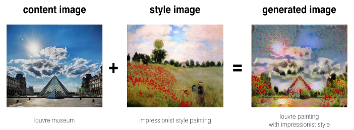
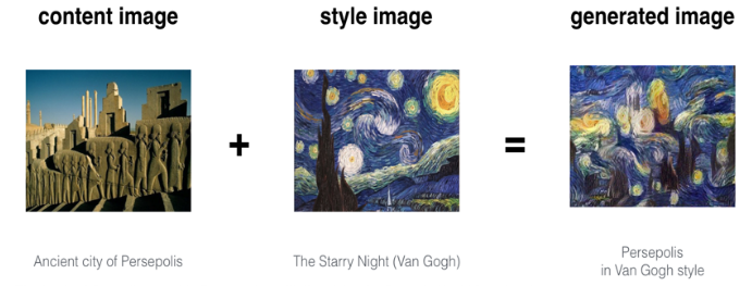
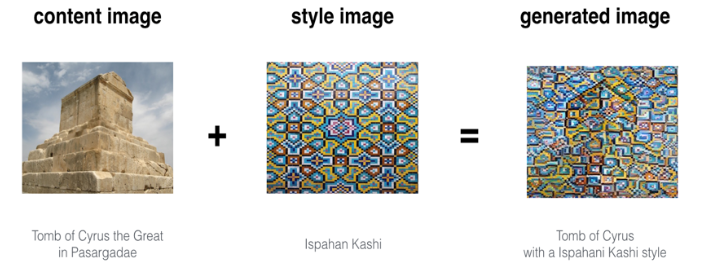
- Neural Style Transfer is an algorithm that given a content image C and a style image S can generate an artistic image
- It uses representations (hidden layer activations) based on a pretrained ConvNet.
- The content cost function is computed using one hidden layer's activations.
- The style cost function for one layer is computed using the Gram matrix of that layer's activations. The overall style cost function is obtained using several hidden layers.
- Optimizing the total cost function results in synthesizing new images.