无监督学习是一种对不含标记的数据建立模型的机器学习范式。
无监督学习应用领域:
- 数据挖掘
- 医学影像
- 股票市场分析
- 计算机视觉
- 市场分析
最常见的无监督学习就是聚类。
聚类的定义:聚类就是对大量未知标注的数据集,按数据的内在相似性将数据集划分为多个类别,使类别内的数据相似度较大而类别间的数据相似度较小
聚类的基本思想:
给定一个有N个对象的数据集,划分聚类技术将构 造数据的k个划分,每一个划分代表一个簇, k≤n。也就是说,聚类将数据划分为k个簇,而且 这k个划分满足下列条件:
1. 每一个簇至少包含一个对象
2. 每一个对象属于且仅属于一个簇
基本思想:对于给定的k,算法首先给出一个初始的划分方法,以后通过反复迭代的方法改变划分, 使得每一次改进之后的划分方案都较前一次更好。
K-means 算法
1. Clustering 中的经典算法,数据挖掘十大经典算法之一。K-means算法,也被称为k-平均或k-均值,是一种 得到最广泛使用的聚类算法,或者成为其他聚类算法的基础。
2. 算法接受参数 k ;然后将事先输入的n个数据对象划分为 k个聚类以便使得所获得的聚类满足:同一聚类中的对象相似度较高;而不同聚类中的对象相似度较小。
3. 算法思想: 以空间中k个点为中心进行聚类,对最靠近他们的对象归类。通过迭代的方法,逐次更新各聚类中心的值,直至得到最好的聚类结果
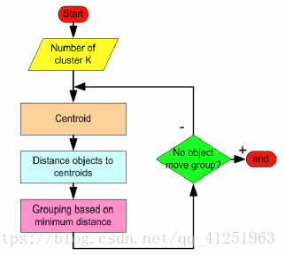
4. 算法描述:
      (1)适当选择c个类的初始中心;
      (2)在第k次迭代中,对任意一个样本,求其到c各中心的距离,将该样本归到距离最短的中心所在的类;
      (3)利用均值等方法更新该类的中心值;
      (4)对于所有的c个聚类中心,如果利用(2)(3)的迭代法更新后,值保持不变,则迭代结束,否则继续迭代。
5.算法流程:
        输入:k, data[n];
      (1) 选择k个初始中心点,例如c[0]=data[0],…c[k-1]=data[k-1];
      (2) 对于data[0]….data[n], 分别与c[0]…c[k-1]比较,假定与c[i]差值最少,就标记为i;
      (3) 对于所有标记为i点,重新计算c[i]={ 所有标记为i的data[j]之和}/标记为i的个数;
      (4) 重复(2)(3),直到所有c[i]值的变化小于给定阈值。
使用《Python机器学习经典实例》一书中kmeans代码展示:
utilities.py
import numpy as np
import matplotlib.pyplot as plt
from sklearn import cross_validation

# Load multivar data in the input file
def load_data(input_file):
    X = []
    with open(input_file, 'r') as f:
        for line in f.readlines():
            data = [float(x) for x in line.split(',')]
            X.append(data)

    return np.array(X)

# Plot the classifier boundaries on input data
def plot_classifier(classifier, X, y, title='Classifier boundaries', annotate=False):
    # define ranges to plot the figure
    x_min, x_max = min(X[:, 0]) - 1.0, max(X[:, 0]) + 1.0
    y_min, y_max = min(X[:, 1]) - 1.0, max(X[:, 1]) + 1.0

    # denotes the step size that will be used in the mesh grid
    step_size = 0.01

    # define the mesh grid
    x_values, y_values = np.meshgrid(np.arange(x_min, x_max, step_size), np.arange(y_min, y_max, step_size))

    # compute the classifier output
    mesh_output = classifier.predict(np.c_[x_values.ravel(), y_values.ravel()])

    # reshape the array
    mesh_output = mesh_output.reshape(x_values.shape)

    # Plot the output using a colored plot
    plt.figure()

    # Set the title
    plt.title(title)

    # choose a color scheme you can find all the options
    # here: http://matplotlib.org/examples/color/colormaps_reference.html
    plt.pcolormesh(x_values, y_values, mesh_output, cmap=plt.cm.Set1)

    # Overlay the training points on the plot
    plt.scatter(X[:, 0], X[:, 1], c=y, edgecolors='black', linewidth=2, cmap=plt.cm.Set1)

    # specify the boundaries of the figure
    plt.xlim(x_values.min(), x_values.max())
    plt.ylim(y_values.min(), y_values.max())

    # specify the ticks on the X and Y axes
    plt.xticks(())
    plt.yticks(())

    if annotate:
        for x, y in zip(X[:, 0], X[:, 1]):
            # Full documentation of the function available here:
            # http://matplotlib.org/api/text_api.html#matplotlib.text.Annotation
            plt.annotate(
                '(' + str(round(x, 1)) + ',' + str(round(y, 1)) + ')',
                xy = (x, y), xytext = (-15, 15),
                textcoords = 'offset points',
                horizontalalignment = 'right',
                verticalalignment = 'bottom',
                bbox = dict(boxstyle = 'round,pad=0.6', fc = 'white', alpha = 0.8),
                arrowprops = dict(arrowstyle = '-', connectionstyle = 'arc3,rad=0'))

# Print performance metrics
def print_accuracy_report(classifier, X, y, num_validations=5):
    accuracy = cross_validation.cross_val_score(classifier,
            X, y, scoring='accuracy', cv=num_validations)
    print ("Accuracy: " + str(round(100*accuracy.mean(), 2)) + "%")

    f1 = cross_validation.cross_val_score(classifier,
            X, y, scoring='f1_weighted', cv=num_validations)
    print ("F1: " + str(round(100*f1.mean(), 2)) + "%")

    precision = cross_validation.cross_val_score(classifier,
            X, y, scoring='precision_weighted', cv=num_validations)
    print ("Precision: " + str(round(100*precision.mean(), 2)) + "%")

    recall = cross_validation.cross_val_score(classifier,
            X, y, scoring='recall_weighted', cv=num_validations)
    print ("Recall: " + str(round(100*recall.mean(), 2)) + "%")
kmeans.py
import numpy as np
import matplotlib.pyplot as plt
from sklearn import metrics
from sklearn.cluster import KMeans
import utilities
# Load data加载数据
data = utilities.load_data('data_multivar.txt')
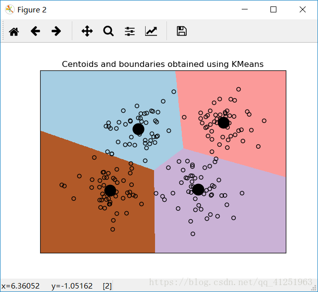
num_clusters = 4#定义集群数量
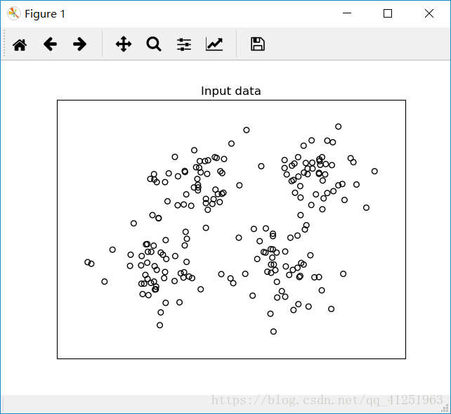
# Plot data画出输入数据
plt.figure()
plt.scatter(data[:,0], data[:,1], marker='o',
facecolors='none', edgecolors='k', s=30)
x_min, x_max = min(data[:, 0]) - 1, max(data[:, 0]) + 1
y_min, y_max = min(data[:, 1]) - 1, max(data[:, 1]) + 1
plt.title('Input data')
plt.xlim(x_min, x_max)
plt.ylim(y_min, y_max)
plt.xticks(())
plt.yticks(())
# Train the model训练模型
kmeans = KMeans(init='k-means++', n_clusters=num_clusters, n_init=10)
kmeans.fit(data)
#可视化边界
# Step size of the mesh,设置网格数据的步长
step_size = 0.01
# Plot the boundaries画出边界
x_min, x_max = min(data[:, 0]) - 1, max(data[:, 0]) + 1
y_min, y_max = min(data[:, 1]) - 1, max(data[:, 1]) + 1
x_values, y_values = np.meshgrid(np.arange(x_min, x_max, step_size), np.arange(y_min, y_max, step_size))
# Predict labels for all points in the mesh预测网格中所有数据点的标记
predicted_labels = kmeans.predict(np.c_[x_values.ravel(), y_values.ravel()])
# Plot the results画出结果
predicted_labels = predicted_labels.reshape(x_values.shape)
plt.figure()
plt.clf()
plt.imshow(predicted_labels, interpolation='nearest',
extent=(x_values.min(), x_values.max(), y_values.min(), y_values.max()),
cmap=plt.cm.Paired,
aspect='auto', origin='lower')
plt.scatter(data[:,0], data[:,1], marker='o',
facecolors='none', edgecolors='k', s=30)
#把中心点画在图形上
centroids = kmeans.cluster_centers_
plt.scatter(centroids[:,0], centroids[:,1], marker='o', s=200, linewidths=3,
color='k', zorder=10, facecolors='black')
x_min, x_max = min(data[:, 0]) - 1, max(data[:, 0]) + 1
y_min, y_max = min(data[:, 1]) - 1, max(data[:, 1]) + 1
plt.title('Centoids and boundaries obtained using KMeans')
plt.xlim(x_min, x_max)
plt.ylim(y_min, y_max)
plt.xticks(())
plt.yticks(())
plt.show()
运行代码后,可以看到下面的图形:
K-means聚类方法总结
优点:
- 是解决聚类问题的一种经典算法,简单、快速
- 对处理大数据集,该算法保持可伸缩性和高效率
- 当结果簇是密集的,它的效果较好
缺点:
- 在簇的平均值可被定义的情况下才能使用,可能不适用 于某些应用
- 必须事先给出k(要生成的簇的数目),而且对初值敏感,对于不同的初始值,可能会导致不同结果。
- 不适合于发现非凸形状的簇或者大小差别很大的簇
- 对躁声和孤立点数据敏感
可作为其他聚类方法的基础算法,如谱聚类