【机器学习实战】降维方法的sklearn实现----PCA和LDA

利用sklearn库来给PCA和LDA做一个比较。首先先了解一下这两个库，然后通过(iris)鸢尾花数据集来进行实践操作。

【PCA】

主要参数：

n_components
int, float, None or string
这个参数类型有int型，float型，string型，默认为None。
它的作用是指定PCA降维后的特征数(也就是降维后的维度)。
若取默认(None)，则n_components==min(n_samples, n_features)，即降维后特征数取样本数和原有特征数之间较小的那个；
若n_components}设置为‘mle’并且svd_solver设置为‘full’则使用MLE算法根据特征的方差分布自动去选择一定数量的主成分特征来降维；
若 $0<$ n_components $<1$ 并且svd_solver设置为‘full’，则n_components为主成分方差的阈值；
若n_components $\ge1$ ，则降维后的特征数为n_components；
若svd_solver设置为‘arpack’，则n_components不能等于n_features。
copy
bool (default True)
在运行算法时，将原始训练数据复制一份。参数为bool型，默认是True，传给fit的原始训练数据X不会被覆盖；若为False，则传给fit后，原始训练数据X会被覆盖。
whiten
bool, optional (default False)
是否对降维后的数据的每个特征进行归一化。参数为bool型，默认是False。
svd_solver
string {‘auto’, ‘full’, ‘arpack’, ‘randomized’}
指定奇异值分解SVD的方法，参数为string类型，可选择‘auto’，‘full’，
‘arpack’，‘randomized’。默认是‘auto’。‘auto’适用于输入数据大于500 $\times$ 500且要提取的成分低于最小维数数据的80%。
$\color{red}{注：前面的PCA方法那篇中，对PCA算法的描述是用特征值分解方法，}$
$\color{red}{由于特征分解是奇异值分解SVD的一个特例，实际应用时可以基于奇异}$
$\color{red}{值分解来实现。}$

主要属性：

components_
array, shape (n_components, n_features)
降维后各主成分方向，并按照各主成分的方差值大小排序。
explained_variance_
array, shape (n_components,)
降维后各主成分的方差值，方差值越大，越主要。
explained_variance_ratio_
array, shape (n_components,)
降维后的各主成分的方差值占总方差值的比例，比例越大，则越主要。
singular_values_
array, shape (n_components,)
奇异值分解得到的前n_components个最大的奇异值。

主要方法:

fit(X,y=None)
用训练数据X训练模型，由于PCA是无监督降维，因此y=None。
transform(X,y=None)
对X进行降维。
fit_transform(X)
用训练数据X训练模型，并对X进行降维。相当于先用fit(X)，再用transform(X)。
inverse_transform(X)
将降维后的数据转换成原始数据。

【LinearDiscriminantAnalysis】

主要参数：

solver
string, optional
求LDA超平面特征矩阵使用的方法，参数类型为string，可选‘svd’、‘lsqr’和‘eigen’，默认选‘svd’。
‘svd’：奇异值分解，不计算协方差矩阵，因此适用于具有大量特征的数据集；
‘lsqr’：最小二乘法，可与正则化一起使用；
‘eigen’：特征值分解，可与正则化一起使用，适用于特征数不多的数据集。
shrinkage
string or float, optional
正则化参数，可以增强LDA分类的泛化能力。若是只用LDA降维，可以不用。参数类型为string或float(0~1之间)，默认是None。
None：不进行正则化；
‘auto’：用Ledoit-Wolf引理自动决定是否使用正则化；
float(0~1之间)：给定正则化参数
正则化只在solver选择‘lsqr’，‘eigen’时有用。
priors
array, optional, shape (n_classes,)
类别权重，用于分类问题时。若是只用LDA降维，可以不用。参数类型为array，大小为类别个数n_classes。
n_components
int, optional
它的作用是指定LDA降维后的特征数(也就是降维后的维度)。参数类型为int，默认为None，1 $\le$ n_components $<$ n_classes-1。若是不做降维，则不设置，用默认即可。

主要属性：

coef_
array, shape (n_features,) or (n_classes, n_features)
特征系数

intercept_
array, shape (n_features,)
偏置

covariance_
array-like, shape (n_features, n_features)
协方差矩阵

explained_variance_ratio_
array, shape (n_components,)
降维后的各主成分的方差值占总方差值的比例，比例越大，则越主要。只在solver选择‘svd’和‘eigen’的时候有用。

主要方法:

与PCA的类似，不过多了predict(X)、decision_function(X)等用于分类问题的方法。

【实践】

导入库：

##用于3D可视化
from mpl_toolkits.mplot3d import Axes3D
##用于可视化图表
import matplotlib.pyplot as plt
##用于做科学计算
import numpy as np
##用于做数据分析
import pandas as pd
##用于加载数据或生成数据等
from sklearn import datasets
##导入PCA库
from sklearn.decomposition import PCA
##导入LDA库
from sklearn.discriminant_analysis import LinearDiscriminantAnalysis

导入数据集：

这次实践就使用iris(鸢尾花)数据集。

iris = datasets.load_iris()
iris_X = iris.data   ##获得数据集中的输入
iris_y = iris.target ##获得数据集中的输出，即标签(也就是类别)
print(iris_X.shape)
print(iris.feature_names)
print(iris.target_names)

输出为：

(150, 4)
['sepal length (cm)', 'sepal width (cm)', 'petal length (cm)', 'petal width (cm)']
['setosa' 'versicolor' 'virginica']

可以看出，iris数据集共有150个样本，每个样本有四个特征(四维)，分别是萼片长度(sepal length)，萼片宽度(sepal width)，花瓣长度(petal length)，花瓣宽度(petal width)。
标签有三种，分别是setosa，versicolor和virginica。

降维：

【PCA】

##加载PCA模型并训练、降维
model_pca = PCA(n_components=3)
X_pca = model_pca.fit(iris_X).transform(iris_X)
print(iris_X.shape)
print(iris_X[0:5])
print(X_pca.shape)
print(X_pca[0:5])

输出为:

(150, 4)
[[ 5.1  3.5  1.4  0.2]
 [ 4.9  3.   1.4  0.2]
 [ 4.7  3.2  1.3  0.2]
 [ 4.6  3.1  1.5  0.2]
 [ 5.   3.6  1.4  0.2]]
(150, 3)
[[-2.68420713  0.32660731 -0.02151184]
 [-2.71539062 -0.16955685 -0.20352143]
 [-2.88981954 -0.13734561  0.02470924]
 [-2.7464372  -0.31112432  0.03767198]
 [-2.72859298  0.33392456  0.0962297 ]]

可以发现原本为四维的样本变为了三维的。让我们分别看看四维和三维时的方差分布。
四维时：

model_pca = PCA(n_components=4)
X_pca = model_pca.fit(iris_X).transform(iris_X)
print("各主成分方向：\n",model_pca.components_)
print("各主成分的方差值：",model_pca.explained_variance_)
print("各主成分的方差值与总方差之比：",model_pca.explained_variance_ratio_)
print("奇异值分解后得到的特征值：",model_pca.singular_values_)
print("主成分数：",model_pca.n_components_)

输出为：

各主成分方向：
 [[ 0.36158968 -0.08226889  0.85657211  0.35884393]
 [ 0.65653988  0.72971237 -0.1757674  -0.07470647]
 [-0.58099728  0.59641809  0.07252408  0.54906091]
 [ 0.31725455 -0.32409435 -0.47971899  0.75112056]]
各主成分的方差值： [ 4.22484077  0.24224357  0.07852391  0.02368303]
各主成分的方差值与总方差之比： [ 0.92461621  0.05301557  0.01718514  0.00518309]
奇异值分解后得到的特征值： [ 25.08986398   6.00785254   3.42053538   1.87850234]
主成分数： 4

三维时：

model_pca = PCA(n_components=3)
X_pca = model_pca.fit(iris_X).transform(iris_X)
print("降维后各主成分方向：\n",model_pca.components_)
print("降维后各主成分的方差值：",model_pca.explained_variance_)
print("降维后各主成分的方差值与总方差之比：",model_pca.explained_variance_ratio_)
print("奇异值分解后得到的特征值：",model_pca.singular_values_)
print("降维后主成分数：",model_pca.n_components_)

输出为：

降维后各主成分方向：
 [[ 0.36158968 -0.08226889  0.85657211  0.35884393]
 [ 0.65653988  0.72971237 -0.1757674  -0.07470647]
 [-0.58099728  0.59641809  0.07252408  0.54906091]]
降维后各主成分的方差值： [ 4.22484077  0.24224357  0.07852391]
降维后各主成分的方差值与总方差之比： [ 0.92461621  0.05301557  0.01718514]
奇异值分解后得到的特征值： [ 25.08986398   6.00785254   3.42053538]
降维后主成分数： 3

我们可以看出从四维降到三维，也就是将四维时，主成分方差值(方差值与总方差之比)最小的那个成分给去掉了。选取的是前三个最大的特征值。
由于降到了三维，我们可以看看用图来看看三维的点的情况。

fig = plt.figure(figsize=(10,8))
ax = Axes3D(fig,rect=[0, 0, 1, 1], elev=30, azim=20)
ax.scatter(X_pca[:, 0], X_pca[:, 1], X_pca[:, 2], marker='o',c=iris_y)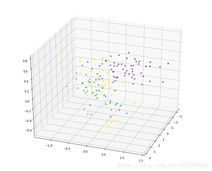

这里写图片描述

我们也可以通过固定elev的值，改变azim的值来看看将这些点投影到各个平面的情况。

fig = plt.figure(figsize=(10,8))
##固定elev=0，改变azim为0，90，180，270
ax = Axes3D(fig,rect=[0, 0, 1, 1], elev=0, azim=0)
ax.scatter(X_pca[:, 0], X_pca[:, 1], X_pca[:, 2], marker='o',c=iris_y)
plt.show()

得到四个图像，可以发现是按这样旋转得到的：
这里写图片描述

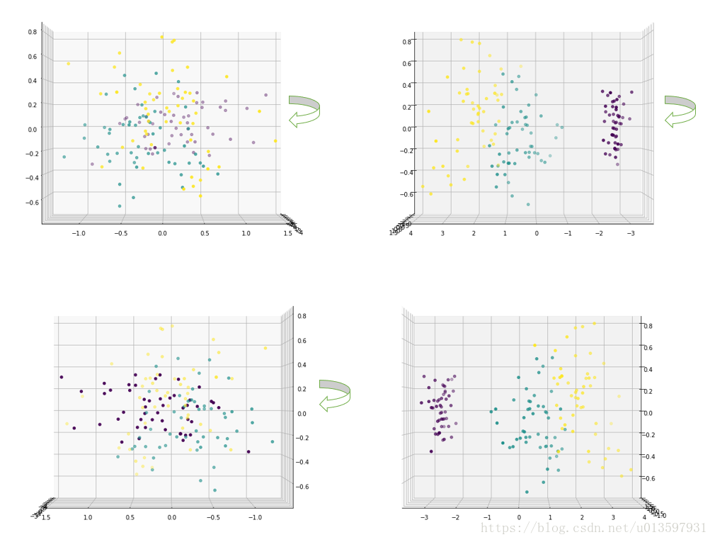
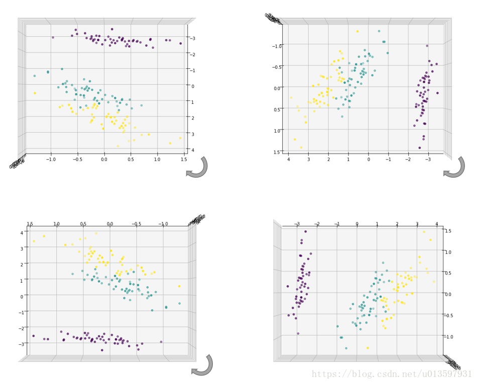
fig = plt.figure(figsize=(10,8))
##固定elev=90，改变azim为0，90，180，270
ax = Axes3D(fig,rect=[0, 0, 1, 1], elev=90, azim=0)
ax.scatter(X_pca[:, 0], X_pca[:, 1], X_pca[:, 2], marker='o',c=iris_y)
plt.show()

另得到四个图像，发现是按这样旋转得到的：
这里写图片描述

我们还可以在看看降维到二维的情况。

model_pca = PCA(n_components=2)
X_pca = model_pca.fit(iris_X).transform(iris_X)
print("降维后各主成分方向：\n",model_pca.components_)
print("降维后各主成分的方差值：",model_pca.explained_variance_)
print("降维后各主成分的方差值与总方差之比：",model_pca.explained_variance_ratio_)
print("奇异值分解后得到的特征值：",model_pca.singular_values_)
print("降维后主成分数：",model_pca.n_components_)

输出为：

降维后各主成分方向：
 [[ 0.36158968 -0.08226889  0.85657211  0.35884393]
 [ 0.65653988  0.72971237 -0.1757674  -0.07470647]]
降维后各主成分的方差值： [ 4.22484077  0.24224357]
降维后各主成分的方差值与总方差之比： [ 0.92461621  0.05301557]
奇异值分解后得到的特征值： [ 25.08986398   6.00785254]
降维后主成分数： 2

我们可以看出从降到二维，其实就是取了方差值(方差值与总方差之比)最大的前两个主成分。继续画图看看。

fig = plt.figure(figsize=(10,8))
plt.scatter(X_pca[:, 0], X_pca[:, 1],marker='o',c=iris_y)
plt.show()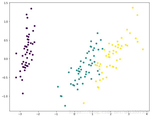

这里写图片描述
和上面有一张从上往下投影的图对应上了，也就是通过降维将那个轴对应的主成分给去掉了。

【LDA】

##载入LDA模型，设置n_components=3
model_lda = LinearDiscriminantAnalysis(n_components=3)
X_lda = model_lda.fit(iris_X, iris_y).transform(iris_X)
print("降维后各主成分的方差值与总方差之比：",model_lda.explained_variance_ratio_)
print("降维前样本数量和维度：",iris_X.shape)
print("降维后样本数量和维度：",X_lda.shape)

输出为：

降维后各主成分的方差值与总方差之比： [ 0.99147248  0.00852752]
降维前样本数量和维度： (150, 4)
降维后样本数量和维度： (150, 2)

我们可以发现并不是按照我设置的维度降维的，而是直接降到了2维。这是因为LDA1的n_component需满足1 $\le$ n_components $\le$ n_classes-1的情况，而这里n_classes为3，因此n_component无论取3还是4都是降维到2。

因此下面这段代码的结果和上面是一样的：

model_lda = LinearDiscriminantAnalysis(n_components=2)
X_lda = model_lda.fit(iris_X, iris_y).transform(iris_X)
print("降维后各主成分的方差值与总方差之比：",model_lda.explained_variance_ratio_)
print("降维前样本数量和维度：",iris_X.shape)
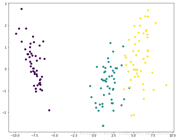
print("降维后样本数量和维度：",X_lda.shape)

得到的各主成分方差值与总方差之比就是前两个主成分。
看看降维后的图像：
这里写图片描述

参考：
1.http://www.cnblogs.com/pinard/p/6243025.html
2.http://www.cnblogs.com/pinard/p/6249328.html
3.http://scikit-learn.org/stable/auto_examples/decomposition/plot_pca_vs_lda.html#sphx-glr-auto-examples-decomposition-plot-pca-vs-lda-py

代码存放于：https://github.com/htshinichi/ML_practice/tree/master