Improvise a Jazz Solo with an LSTM Network

Welcome to your final programming assignment of this week! In this notebook, you will implement a model that uses an LSTM to generate music. You will even be able to listen to your own music at the end of the assignment.

You will learn to:
- Apply an LSTM to music generation. （使用LSTM来生成音乐）
- Generate your own jazz music with deep learning.（通过深度学习来生成自己的Jazz音乐）

Please run the following cell to load all the packages required in this assignment. This may take a few minutes.

from __future__ import print_function
import IPython
import sys
from music21 import *
import numpy as np
from grammar import *
from qa import *
from preprocess import * 
from music_utils import *
from data_utils import *
from keras.models import load_model, Model
from keras.layers import Dense, Activation, Dropout, Input, LSTM, Reshape, Lambda, RepeatVector
from keras.initializers import glorot_uniform
from keras.utils import to_categorical
from keras.optimizers import Adam
from keras import backend as K

1 - Problem statement

You would like to create a jazz music piece specially for a friend’s birthday. However, you don’t know any instruments or music composition. Fortunately, you know deep learning and will solve this problem using an LSTM netwok.

You will train a network to generate novel jazz solos in a style representative of a body of performed work.

1.1 - Dataset

You will train your algorithm on a corpus of Jazz music. Run the cell below to listen to a snippet of the audio from the training set:

（你将在Jazz music中的语料库中训练你的算法，运行下面代码播放训练集中的一小段音乐）

IPython.display.Audio('./data/30s_seq.mp3')

We have taken care of the preprocessing of the musical data to render it in terms of musical “values.” You can informally think of each “value” as a note, which comprises a pitch and a duration. For example, if you press down a specific piano key for 0.5 seconds, then you have just played a note. In music theory, a “value” is actually more complicated than this–specifically, it also captures the information needed to play multiple notes at the same time. For example, when playing a music piece, you might press down two piano keys at the same time (playng multiple notes at the same time generates what’s called a “chord”). But we don’t need to worry about the details of music theory for this assignment. For the purpose of this assignment, all you need to know is that we will obtain a dataset of values, and will learn an RNN model to generate sequences of values.

（我们对音乐数据进行了预处理通过音乐‘值’来解释它。你可以非正式的将每个值看作是一个音符，包括一个高音和一个持续时间。例如，如果你按下一个特定的钢琴键0.5秒，那么你就播放了一个音符。在音乐理论中，‘值’要更加复杂，具体地，它也可以从多个同时播放的音符来捕捉信息。例如，当演奏一段音乐片段，你需要同时按下俩个钢琴的键（同时播放多个音符，产生所谓的‘和弦’）。但我们不需要担心音乐理论的细节。为了完成这个任务，你需要知道的是，我们将获取‘值’的数据集，我们通过学习RNN模型来生成‘值’的序列。）

Our music generation system will use 78 unique values. Run the following code to load the raw music data and preprocess it into values. This might take a few minutes.

（我们音乐生成系统将使用78个不同的‘值’,运行下面的代码来导入原生的音乐数据和将他们预处理成‘值’，这将需要花费几分钟）

X, Y, n_values, indices_values = load_music_utils()  #data/original_metheny.mid
print('shape of X:', X.shape)
print('number of training examples:', X.shape[0]) #训练的样本数
print('Tx (length of sequence):', X.shape[1]) #一段sequence的长度，即x^{1}->x^{30}
print('total # of unique values:', n_values)  #n_values,代表这段音频可以用多少个值来代替
print('Shape of Y:', Y.shape)

Output:

shape of X: (60, 30, 78)
number of training examples: 60
Tx (length of sequence): 30
total # of unique values: 78
Shape of Y: (30, 60, 78)

You have just loaded the following:

X: This is an (m, $T_x$ , 78) dimensional array. We have m training examples, each of which is a snippet of $T_x =30$ musical values. At each time step, the input is one of 78 different possible values, represented as a one-hot vector. Thus for example, X[i,t,:] is a one-hot vector representating the value of the i-th example at time t.

‘X’是一个(m, $T_x$ ,78)维度的矩阵。我们有m个训练样本，每一样本都有 $T_x=30$ 个的音乐‘值’集。在每一个时间步长中，输入为78个不同的可能值中的一个，是一个one-hot vector。因此，对于 X[i,t,:]是一个one-hot向量代表着第i个样本在t时间段的值。

Y: This is essentially the same as X, but shifted one step to the left (to the past). Similar to the dinosaurus assignment, we’re interested in the network using the previous values to predict the next value, so our sequence model will try to predict $y^{\langle t \rangle}$ given $x^{\langle 1\rangle}, \ldots, x^{\langle t \rangle}$ . However, the data in Y is reordered to be dimension $(T_y, m, 78)$ , where $T_y = T_x$ . This format makes it more convenient to feed to the LSTM later.

‘Y’与上一个作业一样，其值与X的值是一样的，但是向左平移了一个位置（即y^{t}=x^{t+1}）。我们使用前一个的输出值来预测下一个值，因此我们的模型将会尝试去预测 $y^{\langle t \rangle}$ ,通过给定 $x^{\langle 1\rangle}, \ldots, x^{\langle t \rangle}$ 。然而，数据 ‘Y’被重新组织成 $（T_y,m,78）$ ，T_y=T_x,这有利于后面的LSTM的输入。（尽管到这里我还不知道为什么）

n_values: The number of unique values in this dataset. This should be 78.

（n_values 在这个数据集上不同值的数量，这里应该是78）

indices_values: python dictionary mapping from 0-77 to musical values.
（indices_values: 使用python字典，将musical values映射成 0-77 的数字）

1.2 - Overview of our model

Here is the architecture of the model we will use. This is similar to the Dinosaurus model you had used in the previous notebook, except that in you will be implementing it in Keras. The architecture is as follows:

（下面的模型是我们将会用到的，这个跟我们前面用到的Dinosaurus model很相似，但是接下来我们会用keras来执行，模型的结构如下所示：）

这里写图片描述

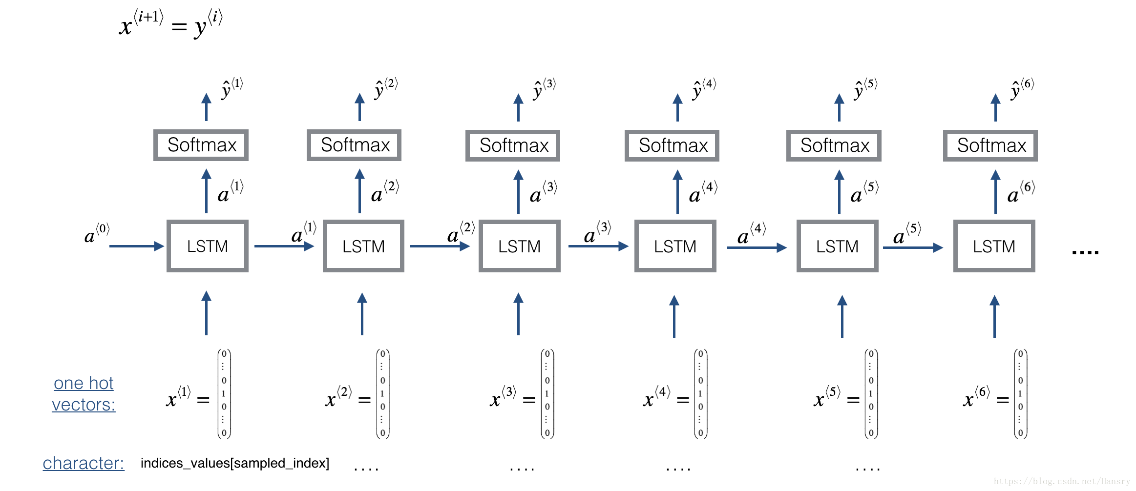
We will be training the model on random snippets of 30 values taken from a much longer piece of music. Thus, we won’t bother to set the first input $x^{\langle 1 \rangle} = \vec{0}$ , which we had done previously to denote the start of a dinosaur name, since now most of these snippets of audio start somewhere in the middle of a piece of music. We are setting each of the snippts to have the same length $T_x = 30$ to make vectorization easier.

2 - Building the model

In this part you will build and train a model that will learn musical patterns. To do so, you will need to build a model that takes in X of shape $(m, T_x, 78)$ and Y of shape $(T_y, m, 78)$ . We will use an LSTM with 64 dimensional hidden states. Lets set n_a = 64.

n_a = 64

Here’s how you can create a Keras model with multiple inputs and outputs. If you’re building an RNN where even at test time entire input sequence $x^{\langle 1 \rangle}, x^{\langle 2 \rangle}, \ldots, x^{\langle T_x \rangle}$ were given in advance, for example if the inputs were words and the output was a label, then Keras has simple built-in functions to build the model. However, for sequence generation, at test time we don’t know all the values of $x^{\langle t\rangle}$ in advance; instead we generate them one at a time using $x^{\langle t\rangle} = y^{\langle t-1 \rangle}$ . So the code will be a bit more complicated, and you’ll need to implement your own for-loop to iterate over the different time steps.

The function djmodel() will call the LSTM layer $T_x$ times using a for-loop, and it is important that all $T_x$ copies have the same weights. I.e., it should not re-initiaiize the weights every time—the $T_x$ steps should have shared weights. The key steps for implementing layers with shareable weights in Keras are:

（函数‘djmodel()’将在 $T_x$ 中的每一个时间步使用for循环来调用LSTM层，值得强调的是所有的 $T_x$ 拥有相同的权重，不应该在每一个时间步重新初始化权重。每一个时间步应该共享其权重。在Keras中执行权重共享的关键步骤为：

Define the layer objects (we will use global variables for this).#定义层对象（我们将会使用全局变量）
Call these objects when propagating the input. #当传播输入的时候调用这些对象

We have defined the layers objects you need as global variables. Please run the next cell to create them. Please check the Keras documentation to make sure you understand what these layers are: Reshape(), LSTM(), Dense().

reshapor = Reshape((1, 78))                        # 实例化一些对象，初始化参数为(1,78) Used in Step 2.B of djmodel(), below
LSTM_cell = LSTM(n_a, return_state = True)         # Used in Step 2.C
densor = Dense(n_values, activation='softmax')     # Used in Step 2.D

Each of reshapor, LSTM_cell and densor are now layer objects, and you can use them to implement djmodel(). In order to propagate a Keras tensor object X through one of these layers, use layer_object(X) (or layer_object([X,Y]) if it requires multiple inputs.). For example, reshapor(X) will propagate X through the Reshape((1,78)) layer defined above.

（每一个‘reshapor’，‘LSTM_cell’和‘densor’现在是layer对象，可以简单的使用它们来执行’djmodel()’这个函数，为了使Keras中的张量X在这些layer中进行传播，可以使用’layer_object(X)’（或者’layer_object([X,Y])’如果需要传播多个输入的时候）例如，’reshapor(X)’ 将会在前面提到的Reshape(1,78)layer中进行传播）

Exercise: Implement djmodel(). You will need to carry out 2 steps:

Create an empty list “outputs” to save the outputs of the LSTM Cell at every time step. （创建空的列表来存储每一个时间步LSTM Cell的输出）

Loop for t∈1,…,Txt∈1,…,Tx : ( for t in range(T_x) )

A. Select the “t”th time-step vector from X. The shape of this selection should be (78,). To do so, create a custom Lambda layer in Keras by using this line of code: (从X中选取第‘t’时间步的向量，该向量维度应该是(78,)，为了实现该效果，利用Kears中的Lambda来实现）

x = Lambda(lambda x: X[:,t,:])(X)

Look over the Keras documentation to figure out what this does. It is creating a “temporary” or “unnamed” function (that’s what Lambda functions are) that extracts out the appropriate one-hot vector, and making this function a Keras Layer object to apply to X.

B. Reshape x to be (1,78). You may find the reshapor() layer (defined below) helpful.
(将向量x reshape成（1,78））

C. Run x through one step of LSTM_cell. Remember to initialize the LSTM_cell with the previous step’s hidden state $a$ and cell state $c$ . Use the following formatting:

(在LSTM_cell传播x，使用上一步的状态 a 和 c 来初始化LSTM_cell)
a, _, c = LSTM_cell(input_x, initial_state=[previous hidden state, previous cell state])
D. Propagate the LSTM’s output activation value through a dense+softmax layer using densor.

E. Append the predicted value to the list of “outputs”

# GRADED FUNCTION: djmodel

def djmodel(Tx, n_a, n_values):
    """
    Implement the model

    Arguments:
    Tx -- length of the sequence in a corpus
    n_a -- the number of activations used in our model
    n_values -- number of unique values in the music data 

    Returns:
    model -- a keras model with the 
    """

    # Define the input of your model with a shape 
    X = Input(shape=(Tx, n_values)) #将输入reshape为(Tx,n_values)

    # Define s0, initial hidden state for the decoder LSTM
    a0 = Input(shape=(n_a,), name='a0')  #将输入reshape为(n_a,)
    c0 = Input(shape=(n_a,), name='c0')  #将输入reshape为(n_a,)
    a = a0
    c = c0

    ### START CODE HERE ### 
    # Step 1: Create empty list to append the outputs while you iterate (≈1 line)
    outputs = []

    # Step 2: Loop
    for t in range(Tx):

        # Step 2.A: select the "t"th time step vector from X. 
        x = Lambda(lambda x: X[:,t,:])(X)
        # Step 2.B: Use reshapor to reshape x to be (1, n_values) (≈1 line)
        x = reshapor(x)
        # Step 2.C: Perform one step of the LSTM_cell
        a, _, c = LSTM_cell(x, initial_state=[a, c])
        # Step 2.D: Apply densor to the hidden state output of LSTM_Cell
        out = densor(a)
        # Step 2.E: add the output to "outputs"
        outputs.append(out)

    # Step 3: Create model instance
    model = Model(input=[X, a0, c0], outputs=outputs) #定义模型

    ### END CODE HERE ###

    return model

Run the following cell to define your model. We will use Tx=30, n_a=64 (the dimension of the LSTM activations), and n_values=78. This cell may take a few seconds to run.

model = djmodel(Tx = 30 , n_a = 64, n_values = 78)  #初始化模型参数,一个样本为30个time-setp,即有30个音符

You now need to compile your model to be trained. We will Adam and a categorical cross-entropy loss.

opt = Adam(lr=0.01, beta_1=0.9, beta_2=0.999, decay=0.01)  #模型优化方式

model.compile(optimizer=opt, loss='categorical_crossentropy', metrics=['accuracy']) #模型编译

Finally, lets initialize a0 and c0 for the LSTM’s initial state to be zero.

m = 60  #这里有60个样本
a0 = np.zeros((m, n_a))
c0 = np.zeros((m, n_a))

Lets now fit the model! We will turn Y to a list before doing so, since the cost function expects Y to be provided in this format (one list item per time-step). So list(Y) is a list with 30 items, where each of the list items is of shape (60,78). Lets train for 100 epochs. This will take a few minutes.

让我们现在 fit 模型！在这样做之前，我们将把Y 变成一个列表，因为代价函数期望Y以这种格式输出（每个时间步一个列表项）。所以list（Y）是一个包含 30 个项目的列表，其中每个列表项目都是形状的（60,78）。让训练100个epochs。这将需要几分钟的时间。

model.fit([X, a0, c0], list(Y), epochs=100)

Output:

Epoch 1/100
60/60 [==============================] - 0s - loss: 4.7687 - dense_1_loss_1: 3.5756 - dense_1_loss_2: 0.7726 - dense_1_loss_3: 0.1530 - dense_1_loss_4: 0.0337 - dense_1_loss_5: 0.0219 - dense_1_loss_6: 0.0147 - dense_1_loss_7: 0.0119 - dense_1_loss_8: 0.0111 - dense_1_loss_9: 0.0094 - dense_1_loss_10: 0.0090 - dense_1_loss_11: 0.0093 - dense_1_loss_12: 0.0080 - dense_1_loss_13: 0.0072 - dense_1_loss_14: 0.0082 - dense_1_loss_15: 0.0081 - dense_1_loss_16: 0.0077 - dense_1_loss_17: 0.0076 - dense_1_loss_18: 0.0077 - dense_1_loss_19: 0.0082 - dense_1_loss_20: 0.0077 - dense_1_loss_21: 0.0080 - dense_1_loss_22: 0.0079 - dense_1_loss_23: 0.0072 - dense_1_loss_24: 0.0077 - dense_1_loss_25: 0.0090 - dense_1_loss_26: 0.0082 - dense_1_loss_27: 0.0086 - dense_1_loss_28: 0.0095 - dense_1_loss_29: 0.0101 - dense_1_loss_30: 0.0000e+00 - dense_1_acc_1: 0.1000 - dense_1_acc_2: 0.7333 - dense_1_acc_3: 0.9667 - dense_1_acc_4: 1.0000 - dense_1_acc_5: 1.0000 - dense_1_acc_6: 1.0000 - dense_1_acc_7: 1.0000 - dense_1_acc_8: 1.0000 - dense_1_acc_9: 1.0000 - dense_1_acc_10: 1.0000 - dense_1_acc_11: 1.0000 - dense_1_acc_12: 1.0000 - dense_1_acc_13: 1.0000 - dense_1_acc_14: 1.0000 - dense_1_acc_15: 1.0000 - dense_1_acc_16: 1.0000 - dense_1_acc_17: 1.0000 - dense_1_acc_18: 1.0000 - dense_1_acc_19: 1.0000 - dense_1_acc_20: 1.0000 - dense_1_acc_21: 1.0000 - dense_1_acc_22: 1.0000 - dense_1_acc_23: 1.0000 - dense_1_acc_24: 1.0000 - dense_1_acc_25: 1.0000 - dense_1_acc_26: 1.0000 - dense_1_acc_27: 1.0000 - dense_1_acc_28: 1.0000 - dense_1_acc_29: 1.0000 - dense_1_acc_30: 0.0000e+00  

... ...
Epoch 100/100
60/60 [==============================] - 0s - loss: 4.4084 - dense_1_loss_1: 3.4707 - dense_1_loss_2: 0.6597 - dense_1_loss_3: 0.1190 - dense_1_loss_4: 0.0204 - dense_1_loss_5: 0.0131 - dense_1_loss_6: 0.0086 - dense_1_loss_7: 0.0071 - dense_1_loss_8: 0.0065 - dense_1_loss_9: 0.0057 - dense_1_loss_10: 0.0052 - dense_1_loss_11: 0.0055 - dense_1_loss_12: 0.0048 - dense_1_loss_13: 0.0043 - dense_1_loss_14: 0.0048 - dense_1_loss_15: 0.0048 - dense_1_loss_16: 0.0046 - dense_1_loss_17: 0.0045 - dense_1_loss_18: 0.0046 - dense_1_loss_19: 0.0049 - dense_1_loss_20: 0.0046 - dense_1_loss_21: 0.0047 - dense_1_loss_22: 0.0047 - dense_1_loss_23: 0.0043 - dense_1_loss_24: 0.0046 - dense_1_loss_25: 0.0053 - dense_1_loss_26: 0.0048 - dense_1_loss_27: 0.0049 - dense_1_loss_28: 0.0056 - dense_1_loss_29: 0.0061 - dense_1_loss_30: 0.0000e+00 - dense_1_acc_1: 0.1000 - dense_1_acc_2: 0.7333 - dense_1_acc_3: 0.9667 - dense_1_acc_4: 1.0000 - dense_1_acc_5: 1.0000 - dense_1_acc_6: 1.0000 - dense_1_acc_7: 1.0000 - dense_1_acc_8: 1.0000 - dense_1_acc_9: 1.0000 - dense_1_acc_10: 1.0000 - dense_1_acc_11: 1.0000 - dense_1_acc_12: 1.0000 - dense_1_acc_13: 1.0000 - dense_1_acc_14: 1.0000 - dense_1_acc_15: 1.0000 - dense_1_acc_16: 1.0000 - dense_1_acc_17: 1.0000 - dense_1_acc_18: 1.0000 - dense_1_acc_19: 1.0000 - dense_1_acc_20: 1.0000 - dense_1_acc_21: 1.0000 - dense_1_acc_22: 1.0000 - dense_1_acc_23: 1.0000 - dense_1_acc_24: 1.0000 - dense_1_acc_25: 1.0000 - dense_1_acc_26: 1.0000 - dense_1_acc_27: 1.0000 - dense_1_acc_28: 1.0000 - dense_1_acc_29: 1.0000 - dense_1_acc_30: 0.0000e+00

从上面可以看出，训练样本有60个样本，对每个样本进行了100次的迭代。

You should see the model loss going down. Now that you have trained a model, lets go on the the final section to implement an inference algorithm, and generate some music!

3 - Generating music

You now have a trained model which has learned the patterns of the jazz soloist. Lets now use this model to synthesize new music.

3.1 - Predicting & Sampling

这里写图片描述

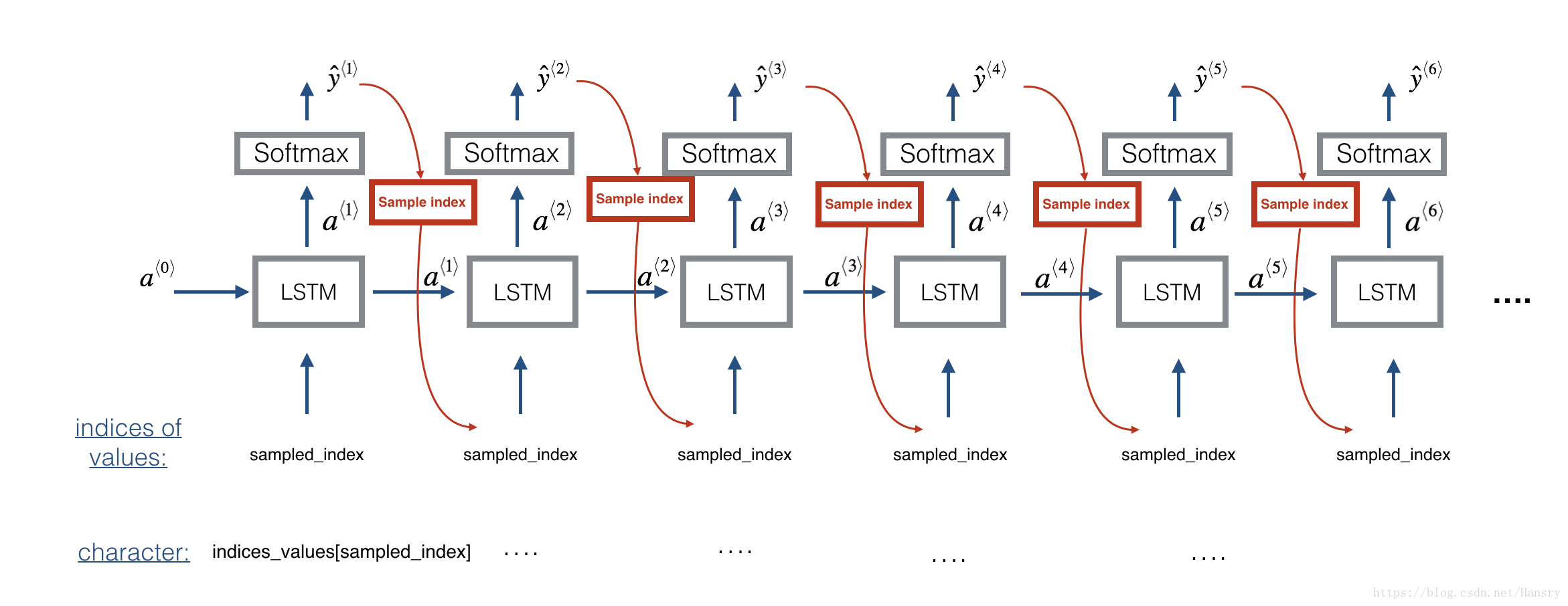
At each step of sampling, you will take as input the activation a and cell state c from the previous state of the LSTM, forward propagate by one step, and get a new output activation as well as cell state. The new activation a can then be used to generate the output, using densor as before.

To start off the model, we will initialize x0 as well as the LSTM activation and and cell value a0 and c0 to be zeros.

(首先先将 x0，a0，c0初始化为0)

Exercise: Implement the function below to sample a sequence of musical values. Here are some of the key steps you’ll need to implement inside the for-loop that generates the $T_y$ output characters:

Step 2.A: Use LSTM_Cell, which inputs the previous step’s c and a to generate the current step’s c and a.

Step 2.B: Use densor (defined previously) to compute a softmax on a to get the output for the current step.

Step 2.C: Save the output you have just generated by appending it to outputs.

Step 2.D: Sample x to the be “out“‘s one-hot version (the prediction) so that you can pass it to the next LSTM’s step. We have already provided this line of code, which uses a Lambda function.

x = Lambda(one_hot)(out)

[Minor technical note: Rather than sampling a value at random according to the probabilities in out, this line of code actually chooses the single most likely note at each step using an argmax.]

(根据“out”的概率，而不是随机抽取一个值，这行代码实际上是在每个步骤中使用argmax选择最可能的音符。)

# GRADED FUNCTION: music_inference_model

def music_inference_model(LSTM_cell, densor, n_values = 78, n_a = 64, Ty = 100):
    """
    Uses the trained "LSTM_cell" and "densor" from model() to generate a sequence of values.

    Arguments:
    LSTM_cell -- the trained "LSTM_cell" from model(), Keras layer object
    densor -- the trained "densor" from model(), Keras layer object
    n_values -- integer, umber of unique values
    n_a -- number of units in the LSTM_cell
    Ty -- integer, number of time steps to generate

    Returns:
    inference_model -- Keras model instance
    """

    # Define the input of your model with a shape 
    x0 = Input(shape=(1, n_values)) #(1,78)

    # Define s0, initial hidden state for the decoder LSTM
    a0 = Input(shape=(n_a,), name='a0') #(64,)
    c0 = Input(shape=(n_a,), name='c0') #(64,)
    a = a0
    c = c0
    x = x0

    ### START CODE HERE ###
    # Step 1: Create an empty list of "outputs" to later store your predicted values (≈1 line)
    outputs = []

    # Step 2: Loop over Ty and generate a value at every time step
    for t in range(Ty):

        # Step 2.A: Perform one step of LSTM_cell (≈1 line)
        a, _, c = LSTM_cell(x, initial_state=[a, c])

        # Step 2.B: Apply Dense layer to the hidden state output of the LSTM_cell (≈1 line)
        out = densor(a)

        # Step 2.C: Append the prediction "out" to "outputs". out.shape = (None, 78) (≈1 line)
        outputs.append(out)

        # Step 2.D: Select the next value according to "out", and set "x" to be the one-hot representation of the
        #           selected value, which will be passed as the input to LSTM_cell on the next step. We have provided 
        #           the line of code you need to do this. 
        x = Lambda(one_hot)(out) #将上一步的输出作为下一步的输入并将其转换为one-hot向量

    # Step 3: Create model instance with the correct "inputs" and "outputs" (≈1 line)
    inference_model = Model(input=[x0, a0, c0], outputs=outputs)

    ### END CODE HERE ###

    return inference_model

Run the cell below to define your inference model. This model is hard coded to generate 50 values.

inference_model = music_inference_model(LSTM_cell, densor, n_values = 78, n_a = 64, Ty = 50)

Finally, this creates the zero-valued vectors you will use to initialize x and the LSTM state variables a and c.

x_initializer = np.zeros((1, 1, 78))
a_initializer = np.zeros((1, n_a))
c_initializer = np.zeros((1, n_a))

Exercise: Implement predict_and_sample(). This function takes many arguments including the inputs [x_initializer, a_initializer, c_initializer]. In order to predict the output corresponding to this input, you will need to carry-out 3 steps:

这个函数拥有许多的参数，其中的输入有x_initializer,a_initializer,c_initializer. 为了使得输出与输入对应，需要执行下面3个步骤：

Use your inference model to predict an output given your set of inputs. The output pred should be a list of length $T_y$ where each element is a numpy-array of shape (1, n_values).

(1.使用inference model来预测给定的输入，输出应该是一个长为 $T_y$ 的列表且每一个元素的shape为（1，n_values））

Convert pred into a numpy array of $T_y$ indices. Each index corresponds is computed by taking the argmax of an element of the pred list. Hint

(2.将‘pred’转换为一个 $T_y$ 索引的numpy数组，每个索引对应的是通过argmax生成的列表中的最大值，即最可能的那个值。)

Convert the indices into their one-hot vector representations. Hint

（3.将索引转换成one-hot向量表示）

# GRADED FUNCTION: predict_and_sample

def predict_and_sample(inference_model, x_initializer = x_initializer, a_initializer = a_initializer, 
                       c_initializer = c_initializer):
    """
    Predicts the next value of values using the inference model.

    Arguments:
    inference_model -- Keras model instance for inference time
    x_initializer -- numpy array of shape (1, 1, 78), one-hot vector initializing the values generation
    a_initializer -- numpy array of shape (1, n_a), initializing the hidden state of the LSTM_cell
    c_initializer -- numpy array of shape (1, n_a), initializing the cell state of the LSTM_cel

    Returns:
    results -- numpy-array of shape (Ty, 78), matrix of one-hot vectors representing the values generated
    indices -- numpy-array of shape (Ty, 1), matrix of indices representing the values generated
    """

    ### START CODE HERE ###
    # Step 1: Use your inference model to predict an output sequence given x_initializer, a_initializer and c_initializer.
    pred = inference_model.predict([x_initializer, a_initializer, c_initializer])
    # Step 2: Convert "pred" into an np.array() of indices with the maximum probabilities
    indices = np.argmax(np.array(pred),axis=-1)
    # Step 3: Convert indices to one-hot vectors, the shape of the results should be (1, )
    results = to_categorical(indices, num_classes=x_initializer.shape[-1])
    ### END CODE HERE ###

    return results, indices

results, indices = predict_and_sample(inference_model, x_initializer, a_initializer, c_initializer)
print("np.argmax(results[12]) =", np.argmax(results[12]))
print("np.argmax(results[17]) =", np.argmax(results[17]))
print("list(indices[1:18]) =", list(indices[1:18]))

3.3 - Generate music

Finally, you are ready to generate music. Your RNN generates a sequence of values. The following code generates music by first calling your predict_and_sample() function. These values are then post-processed into musical chords (meaning that multiple values or notes can be played at the same time).

最后，你已经准备去生成音乐了。你的RNN生成一个序列的value，下面的代码通过调用‘predict_and_sample（）’形成音乐。这些values然后处理成音乐的和弦（意味着可以同时播放多个values和符号）

Most computational music algorithms use some post-processing because it is difficult to generate music that sounds good without such post-processing. The post-processing does things such as clean up the generated audio by making sure the same sound is not repeated too many times, that two successive notes are not too far from each other in pitch, and so on. One could argue that a lot of these post-processing steps are hacks; also, a lot the music generation literature has also focused on hand-crafting post-processors, and a lot of the output quality depends on the quality of the post-processing and not just the quality of the RNN. But this post-processing does make a huge difference, so lets use it in our implementation as well.

大多数音乐计算算法使用了一些后处理因为如果没有后处理的话很难生成好听的音乐。后处理确保相同的声音不重复多次，保证两个连续的音符在音高中彼此相距不太远。有人可能会说，很多这些后处理步骤都是黑客行为;另外，很多音乐创作文献也专注于手工制作后期处理器，很多输出质量取决于后期处理的质量，而不仅仅取决于 RNN 的质量。但是这个后期处理确实有很大的不同，所以我们也可以在我们的实现中使用它。
Lets make some music!

Run the following cell to generate music and record it into your out_stream. This can take a couple of minutes.

out_stream = generate_music(inference_model)

Output：

Predicting new values for different set of chords.
Generated 51 sounds using the predicted values for the set of chords ("1") and after pruning
Generated 51 sounds using the predicted values for the set of chords ("2") and after pruning
Generated 51 sounds using the predicted values for the set of chords ("3") and after pruning
Generated 51 sounds using the predicted values for the set of chords ("4") and after pruning
Generated 51 sounds using the predicted values for the set of chords ("5") and after pruning
Your generated music is saved in output/my_music.midi

To listen to your music, click File->Open… Then go to “output/” and download “my_music.midi”. Either play it on your computer with an application that can read midi files if you have one, or use one of the free online “MIDI to mp3” conversion tools to convert this to mp3.

As reference, here also is a 30sec audio clip we generated using this algorithm.

IPython.display.Audio('./data/30s_trained_model.mp3')