1.随机梯度下降法(SGD)
随机梯度下降法是用来求参数的优化算法,具体算法不过多阐述,此处采用线性拟合来实现SGD,同时使用TensorFlow进行计算,具体思路注释写的较为清楚,直接附上代码:
import tensorflow as tf
import numpy as np
import matplotlib.pyplot as plt
#权重
W=0.3
#偏置
b=0.8
np.random.seed(10)
#构建训练数据集
def get_train_data(data_length):
train_arr=[]
for i in range(data_length):
tr_x=np.random.uniform(0.0,1.0)
#给予区间为[-0.02,0.02]的抖动
tr_y=tr_x*W+b+np.random.uniform(-0.02,0.02)
#将输入和输出保存至训练集
train_arr.append([tr_x,tr_y])
return train_arr
#构建验证数据集
def get_validate_data(data_length):
validate_arr=[]
for i in range(data_length):
va_x=np.random.uniform(0.0,1.0)
va_y=va_x*W+b+np.random.uniform(-0.02,0.02)
validate_arr.append([va_x,va_y])
return validate_arr
#获取200组输入数据
trainData=get_train_data(200)
#获取输入x和结果y
trainx=[v[0] for v in trainData]
trainy=[v[1] for v in trainData]
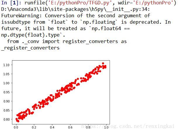
#做出原图
plt.plot(trainx,trainy,'ro',label='train data')
plt.show()
#TF训练
sess=tf.Session()
#赋予权重W随机值
W=tf.Variable(tf.random_normal([1]),name='weight')
b=tf.Variable(tf.random_normal([1]),name='bias')
#使用X、Y占位符
X=tf.placeholder(tf.float32,shape=[None])
Y=tf.placeholder(tf.float32,shape=[None])
hypothesis=X*W+b
#loss function(损失函数)
#平方差函数
cost=tf.reduce_mean(tf.square(hypothesis-Y))
'''
用来显示标量信息
'''
tf.summary.scalar('cost_linear',cost)
#Minimize
#进行优化
optimizer=tf.train.GradientDescentOptimizer(learning_rate=0.009)
train=optimizer.minimize(cost)
'''
merge_all 可以将所有summary全部保存到磁盘,以便tensorboard显示。
如果没有特殊要求,一般用这一句就可一显示训练时的各种信息了。
'''
merged=tf.summary.merge_all()
sess.run(tf.global_variables_initializer())
#将sess图写入文件中
write=tf.summary.FileWriter('log',sess.graph)
#训练2000次
for step in range(2001):
cost_val,merg,W_val,b_val,_=sess.run([cost,merged,W,b,train],
feed_dict={X:trainx,
Y:trainy})
if step % 20==0:
print(step,cost_val,W_val,b_val)
#将每一步和图信息保存
write.add_summary(merg,step)
write.close()
#plt.plot(trainx,trainy,'ro',label='train data')
#做出训练图像
plt.plot(trainx,sess.run(hypothesis,feed_dict={X:trainx,
Y:trainy}),label='train result')
#显示图例
plt.legend()
plt.show()损失函数使用平方差函数进行度量,经过2000次迭代,运行结果为:
0 4.331622 [-0.652807] [-0.7690222]
20 1.7611761 [-0.35204175] [-0.17788434]
40 0.71652895 [-0.15930393] [0.19845636]
60 0.29195884 [-0.03545507] [0.4378772]
80 0.11938576 [0.04445574] [0.59002405]
100 0.049223986 [0.09633496] [0.68654543]
120 0.020682896 [0.13032326] [0.7476167]
140 0.009057453 [0.15288574] [0.786099]
160 0.004307573 [0.16814426] [0.8101914]
180 0.0023530128 [0.17872691] [0.8251203]
200 0.0015355434 [0.18630955] [0.8342169]
220 0.0011812018 [0.19196095] [0.83960503]
240 0.0010160565 [0.19636281] [0.8426383]
260 0.0009287362 [0.1999502] [0.84417945]
280 0.00087394175 [0.20300078] [0.8447782]
300 0.0008332224 [0.20569208] [0.8447845]
320 0.0007990418 [0.20813756] [0.84442186]
340 0.00076830183 [0.21040995] [0.84383225]
360 0.00073970767 [0.21255597] [0.84310585]
380 0.0007127009 [0.21460575] [0.8423002]
400 0.0006870223 [0.21657889] [0.84145164]
420 0.0006625359 [0.21848822] [0.8405833]
440 0.0006391577 [0.22034223] [0.83970976]
460 0.0006168266 [0.22214669] [0.83884]
480 0.0005954896 [0.22390564] [0.8379797]
500 0.00057510135 [0.22562185] [0.8371323]
520 0.00055561884 [0.22729748] [0.83629984]
540 0.0005370013 [0.2289342] [0.83548343]
560 0.0005192104 [0.23053333] [0.83468366]
580 0.00050220994 [0.23209599] [0.83390087]
600 0.00048596383 [0.23362328] [0.83313495]
620 0.0004704391 [0.23511603] [0.8323858]
640 0.00045560338 [0.23657516] [0.8316532]
660 0.00044142597 [0.23800144] [0.8309368]
680 0.0004278783 [0.23939565] [0.8302364]
700 0.0004149319 [0.24075852] [0.82955164]
720 0.00040256046 [0.24209076] [0.8288823]
740 0.0003907386 [0.24339306] [0.8282279]
760 0.00037944122 [0.24466614] [0.8275882]
780 0.00036864527 [0.24591063] [0.82696277]
800 0.0003583285 [0.24712719] [0.82635146]
820 0.0003484699 [0.24831645] [0.8257538]
840 0.00033904883 [0.249479] [0.8251696]
860 0.000330046 [0.25061545] [0.8245985]
880 0.00032144293 [0.2517264] [0.82404023]
900 0.00031322165 [0.2528124] [0.8234945]
920 0.00030536592 [0.25387394] [0.82296103]
940 0.00029785887 [0.25491166] [0.8224395]
960 0.00029068452 [0.25592616] [0.8219297]
980 0.00028382873 [0.2569179] [0.8214313]
1000 0.00027727737 [0.25788733] [0.8209441]
1020 0.00027101676 [0.25883502] [0.8204678]
1040 0.00026503406 [0.25976145] [0.82000226]
1060 0.0002593171 [0.26066706] [0.8195471]
1080 0.00025385374 [0.26155233] [0.8191022]
1100 0.00024863315 [0.26241776] [0.8186673]
1120 0.00024364427 [0.26326373] [0.8182422]
1140 0.0002388769 [0.26409075] [0.8178266]
1160 0.00023432102 [0.26489916] [0.8174203]
1180 0.00022996707 [0.26568952] [0.81702316]
1200 0.0002258068 [0.26646206] [0.81663495]
1220 0.0002218312 [0.26721725] [0.81625545]
1240 0.00021803215 [0.26795548] [0.8158844]
1260 0.00021440185 [0.26867715] [0.8155218]
1280 0.00021093212 [0.26938266] [0.8151671]
1300 0.00020761647 [0.27007234] [0.8148204]
1320 0.0002044484 [0.2707465] [0.8144817]
1340 0.00020142079 [0.27140558] [0.8141505]
1360 0.00019852784 [0.2720498] [0.8138268]
1380 0.00019576306 [0.2726796] [0.8135103]
1400 0.00019312126 [0.27329522] [0.81320095]
1420 0.00019059677 [0.27389702] [0.8128985]
1440 0.00018818416 [0.27448532] [0.8126029]
1460 0.00018587877 [0.27506042] [0.8123139]
1480 0.00018367577 [0.27562255] [0.8120314]
1500 0.0001815708 [0.27617207] [0.81175524]
1520 0.00017955857 [0.2767094] [0.81148523]
1540 0.00017763514 [0.27723482] [0.8112212]
1560 0.00017579742 [0.27774832] [0.8109631]
1580 0.00017404192 [0.27825016] [0.8107109]
1600 0.0001723644 [0.2787407] [0.8104643]
1620 0.00017076127 [0.27922028] [0.8102234]
1640 0.00016922936 [0.27968907] [0.8099878]
1660 0.0001677654 [0.28014734] [0.8097575]
1680 0.00016636639 [0.28059533] [0.80953234]
1700 0.00016502957 [0.28103325] [0.8093123]
1720 0.0001637521 [0.28146136] [0.8090971]
1740 0.00016253124 [0.28187984] [0.80888677]
1760 0.00016136453 [0.28228897] [0.80868113]
1780 0.0001602498 [0.2826889] [0.8084802]
1800 0.0001591845 [0.2830798] [0.8082838]
1820 0.00015816656 [0.28346193] [0.80809176]
1840 0.00015719362 [0.28383553] [0.807904]
1860 0.000156264 [0.28420073] [0.8077205]
1880 0.00015537559 [0.28455773] [0.8075411]
1900 0.00015452661 [0.2849067] [0.8073656]
1920 0.0001537153 [0.28524786] [0.8071942]
1940 0.00015294018 [0.28558135] [0.8070266]
1960 0.00015219934 [0.28590736] [0.80686283]
1980 0.00015149127 [0.28622606] [0.8067027]
2000 0.00015081473 [0.28653762] [0.8065461]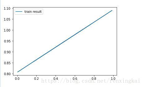
通过结果,可以看到经过2000次迭代,损失函数值为0.00015081473,W值为0.287,b值为0.8265
2.最小二乘法(矩阵表示)
最小二乘法的矩阵表示法如下图:

此处通过TF计算,最终程序的最小二乘法矩阵表达公式为:

代码中注释较为详细,直接附上代码:
import numpy as np
import tensorflow as tf
import matplotlib.pyplot as plt

sess=tf.Session()
#将[0,10]等分100份
x_vals=np.linspace(0,10,100)
#将[0,1]等分100份,同时将y值设置为与x相加(在x的基础上对y值进行计算)
y_vals=x_vals+np.random.normal(0,1,100)

#将x变为矩阵,然后再转置,此时x_vals_column为100*1的矩阵
x_vals_column=np.transpose(np.matrix(x_vals))

#np.matrix生成矩阵,np.repeat为对第一个值的复制
'''
np.repeat(2,3)
Out[8]: array([2, 2, 2])
'''
#将1复制100次,变为1*100的矩阵,再转置-->变为100*1的全1矩阵
ones_column=np.transpose(np.matrix(np.repeat(1,100)))

#合并生成100行,2列,第一列为[0,10]的等分100份值,第二列为全1
A=np.column_stack((x_vals_column,ones_column))
#100行1列
#b为100*1矩阵,值为[0,1)之间100个随机值
b=np.transpose(np.matrix(y_vals))

#定义A,b为常量
A_tensor=tf.constant(A)
b_tensor=tf.constant(b)


#2*100矩阵和100*2矩阵相乘,结果得到2*2矩阵
tA_A=tf.matmul(tf.transpose(A_tensor),A_tensor)
#求tA_A的逆,仍为2*2矩阵
tA_A_inv=tf.matrix_inverse(tA_A)


#2*2矩阵和2*100矩阵相乘,得到2*100矩阵
product=tf.matmul(tA_A_inv,tf.transpose(A_tensor))
#2*100矩阵和100*1矩阵相乘,得到solution为2*1矩阵
solution=tf.matmul(product,b_tensor)
solution_eval=sess.run(solution)


slope=solution_eval[0][0]
y_intercept=solution_eval[1][0]

print('slope:',slope)
print('y_intercept:',y_intercept)

best_fit=[]
#计算最小二乘法之后的预测值
for each in x_vals:
    best_fit.append(slope*each+y_intercept)

#做出原始数据
plt.plot(x_vals,y_vals,'o',label = "Data")
#做出预测值

plt.plot(x_vals,best_fit,'r-',label="Fit line",linewidth=3)
 #图例位置
plt.legend(loc='upper left')
#显示
plt.show()
结果为:
