TensorFlow入门（1）

import tensorflow as tf

hello = tf.constant("hello,tensorflow!")  #创建一个常量
sess = tf.Session()   #启动Tensorflow的Session
print(sess.run(hello))   #调用sess的run方法来启动整个graph
# b'hello,tensorflow!'

a = tf.constant(2)
b = tf.constant(3)
with tf.Session() as sess:
    print("a = 2, b = 3")
    print("Addition with constants:%i"%sess.run(a + b))
    print("Multiplication with constants:%i"%sess.run(a * b))
# a = 2, b = 3
# Addition with constants:5
# Multiplication with constants:6

# 用tensorflow的placeholder来定义变量做类似计算
a = tf.placeholder(tf.int16)
b = tf.placeholder(tf.int16)
add = tf.add(a,b)
mul = tf.multiply(a,b)
with tf.Session() as sess:
    #run every operation with variable input
    print("Addition with variables:%i"% sess.run(add,feed_dict={a:2,b:3}))
    print("Multiplication with variables:%i"%sess.run(mul,feed_dict={a:2,b:3}))
# Addition with variables:5
# Multiplication with variables:6

#线性回归
import tensorflow as tf
import numpy
import matplotlib.pyplot as plt
rng = numpy.random

# Parameters
learning_rate = 0.01
training_epochs = 2000
display_step = 50

# Training Data
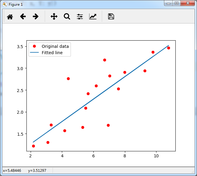
train_X = numpy.asarray([3.3,4.4,5.5,6.71,6.93,4.168,9.779,6.182,7.59,2.167,7.042,10.791,5.313,7.997,5.654,9.27,3.1])
train_Y = numpy.asarray([1.7,2.76,2.09,3.19,1.694,1.573,3.366,2.596,2.53,1.221,2.827,3.465,1.65,2.904,2.42,2.94,1.3])
n_samples = train_X.shape[0]

# tf Graph Input
X = tf.placeholder("float")
Y = tf.placeholder("float")

# Create Model

# Set model weights
W = tf.Variable(rng.randn(), name="weight")
b = tf.Variable(rng.randn(), name="bias")

# Construct a linear model
activation = tf.add(tf.multiply(X, W), b)

# Minimize the squared errors
cost = tf.reduce_sum(tf.pow(activation-Y, 2))/(2*n_samples) #L2 loss
optimizer = tf.train.GradientDescentOptimizer(learning_rate).minimize(cost) #Gradient descent

# Initializing the variables
init = tf.initialize_all_variables()

# Launch the graph
with tf.Session() as sess:
    sess.run(init)

    # Fit all training data
    for epoch in range(training_epochs):
        for (x, y) in zip(train_X, train_Y):
            sess.run(optimizer, feed_dict={X: x, Y: y})

        #Display logs per epoch step
        if epoch % display_step == 0:
            print ("Epoch:", '%04d' % (epoch+1), "cost=", \
                "{:.9f}".format(sess.run(cost, feed_dict={X: train_X, Y:train_Y})), \
                "W=", sess.run(W), "b=", sess.run(b))

    print ("Optimization Finished!")
    print ("cost=", sess.run(cost, feed_dict={X: train_X, Y: train_Y}), \
          "W=", sess.run(W), "b=", sess.run(b))

    #Graphic display
    plt.plot(train_X, train_Y, 'ro', label='Original data')
    plt.plot(train_X, sess.run(W) * train_X + sess.run(b), label='Fitted line')
    plt.legend()
    plt.show()