To talk about the Distance-to-Default, we would like to discuss approaches about the credit risk analytics in econometrics. In econometrics, there are two common approaches to construct a model. One is the structural model, the other is reduced model. The main difference is the structural model is estimated in their theoretically given form, however, as for reduced form model is estimated by the exogenous variables.
In credit analytics fields, it is important to estimate one company's probability of default. And distance-to-default can be used to imply a probability of default. Just as the name implies, probability of default measures the likelihood of an obligor being unable to honor its financial obligation. Distance-to-Default implies the how far a company is away from a default. Typically, a higher probability of default indicates a lower Distance-to-Default.
There are several methods to estimate the Distance-to-Default for a company such as Merton's model, KMV model. KMV is a modified version of Merton's concept, and we will discuss these models later.
Merton Model
Merton model is named after economist Robert C.Merton who has received the 1997's Nobel Prize due to his contribution to Option Pricing Theory. The merton model makes some assumptions which are similar to the option pricing theory.
There are some assumptions of the merton model.
- according to the accounting stardards, assets(V) are the sum of liabilities(K) and equities(E)
- assuming that the interest rate is constant
- assuming that the volatility is constant
- the assets follow a geometric brown motion
- the liabilities can be seen as a single outstanding bond with face value K and maturity T
- debt and equity are frictionless tradeable assets
- a company's default will be seen as its asset value falls below the liability at the end of T
According to its assumptions, it is best when applied to publicly traded companies whose market information and financial statements are available. And the value of the firm can be represented as \[\frac{dV}{V} = \mu dt + \sigma dB_t\]
\(V\) is the value of the firm, \(\mu\) is the drigt of the asset value in the physical measure, and \(\sigma\) is the volatility of the asset value. Equity holders receive the excess value of the firm above the its liabilities. The payoff will be \[E = max(V-K,0)\]
Hence, the equity can be viewed as a European call option on the firm's asset V at a exercise price at K. Then we find the Black-Scholes option pricing formula \[E = VN(d_1)-\mathcal{e}^{-r(T-t)}KN(d_2)\]
where \(r\) is the risk-free rate and \(N(\cdot)\) is the standard normal cumulative distribution function.
\[d_1=\frac{log(\frac{V}{K})+(r+\frac{\sigma^2}{2})(T-t)}{\sigma \sqrt{T-t}}\]
\[d_2=\frac{log(\frac{V}{K})+(r-\frac{\sigma^2}{2})(T-t)}{\sigma \sqrt{T-t}}\]
Following Merton's model, the distance-to-default can be defined as \[DD_t = \frac{log(\frac{V_t}{K})+(\mu-\frac{\sigma^2_A}{2})(T-t)}{\sigma_A\sqrt{T-t}}\]
Based on the definition of default under Merton Model, the probability of default will be \[PD = N(-DD_t)\]
From the assumptions of Merton's model, it is obvious that there are some limitations of Merton Model. Firstly, interest rates and volatility are regarded as constant, which is in conflict with our common sense. Secondly, all liabilities are mapped into a single zero-coupon bond of a maturity of T. In real world, the balance sheet is quite complex and the liabilities are combined with different accounting items such as short liabilities, long-term liabilities and other liabilities. Finally, from the empirical study, the definition of default is not so accurate. Many companies will not default even if its assets value falls below the liabilities.
So I would like to introduce KMV model, which can be seen as a modified version of Merton Model that takes the real world information into account.
KMV Model
KMV model is first introduced by KMV company, a credit analytics company now acquired by Moody's. Based on its proprietary databse, KMV proceded an extension of Merton Model for estimating probability of default and distance to default.
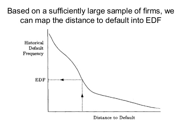
Compared to Merton Model, KMV considered the structure of debt and initiated a concept of default point, which replaces Merton's principal of zero-coupon bond K to a value of the firm's current liabilties plus one half of its long-term debt.\[K = current\ liabilities\ + \ 0.5\times \ longterm\ liabilities\] After the calculation of Distance-to-Default, a default databased is used to derie an empirical distrition relating the distance-to-default to a probability of default. The figure below will give an illustration.
Estimation of Distance-to-Default
As for the KMV model, after given the default point data(from balance sheet), equity data and risk-free rate(from market), we need to estimate the company's asset value and its corresponding volatility. We have already established a formula from the option pricing theory. \[E_t = V_tN(d_1)-\mathcal{e}^{-r(T-t)}KN(d_2)\ \ \ \ \ \ \ (1)\] where
\[d_1=\frac{log(\frac{V_t}{K})+(r+\frac{\sigma^2_A}{2})(T-t)}{\sigma_a \sqrt{T-t}}\]
\[d_2=\frac{log(\frac{V_t}{K})+(r-\frac{\sigma^2_A}{2})(T-t)}{\sigma_A \sqrt{T-t}}\]
It comes to a question, how to esitmate the asset volatility \(\sigma_V\). Typically, there are two possible approaches:
- Using Ito's Lemma(Jones et al 1984)
- Using compound option(Hull, Nelken and White (2004))
I will demonstrate estimation using the Ito's Lemma. We can link the volatility of assets to the volatility of equity by an equation
\[\sigma_E = \frac{V_A}{V_E}\times \frac{\partial V_E}{\partial V_A}\sigma_A \ \ \ \ (2)\]
Given the equation (1) and (2), it comes to solve a nonlinear system of equations
\[f_1(V_E,\sigma_E) = V_AN(d_1)-\mathcal{e}^{-r(T-t)}KN(d_2)-V_E=0\]
\[f_2(V_E,\sigma_E) = \frac{V_A}{V_E}\times \frac{\partial V_E}{\partial V_A}\sigma_A - \sigma_E =0\]
since \[\frac{\partial f_1(V_E,\sigma_E)}{\partial V_A} = N(d_1)-\frac{\partial V_E}{\partial V_A} = 0\]
\(f_2(V_E,\sigma_E)\) can be simplified as
\[f_2(V_E,\sigma_E) = \frac{V_A}{V_E}N(d_1)\sigma_A - \sigma_E =0\]
Our goal is to estimate parameters by solving the equation (1) and (2). Python has provided several optimizer to solve such equations. Take scipy.optimize as an instance, it offers various numerical optimizations and root finding methods. You may refer to https://docs.scipy.org/doc/scipy/reference/optimize.html. Here, we use minimize function to solve such equations.
# import relative modules
import numpy as np
from scipy.stats import norm
from scipy.optimize import minimize
I would like to use real world data to demonstrate the Distance-to-Default parameter calibration. Here, we adopt one dimension estimation and use the default optimization in minimize function. If you are curious about the difference between the one or two dimension estimation and other numerical optimization method, we can try to use different settings.
Here, we would like to use WalMart Inc(the top 1 in Fortune Global 500)
| Variable | Value |
|---|---|
| Current liabilities(Released on 31 Jan 2018) | 78,521 million USD |
| Longterm Debt(Released on 31 Jan 2018) | 32,784 million USD |
| Market Cap(upto 29 June 2018) | 252,740 million USD |
| Volatility of equity(using 1 year return) | 0.0145078 |
| 1 year treausury yield(29 June 2018) | 2.33% |
V_equity = 252740
default_point = 78521+32784/2
rf_rate = 2.33
sigma_equity = 0.145078
T = 1
# One dimension estimation
def equation(x):
    d1 = (np.log(x[0]/default_point) + (rf_rate+x[1]**2/2)*T)/(x[1] * np.sqrt(T))
    d2 = d1 - x[1] * np.sqrt(T)
    res1 = x[0] * norm.cdf(d1) - np.exp(-rf_rate*T) * default_point * norm.cdf(d2) - V_equity
    res2 = x[0] * norm.cdf(d1) * x[1] - V_equity * sigma_equity
    return(res1**2+res2**2)
result = minimize(equation, [252740,0.145078])
result fun: 3.884352384861794e-06
hess_inv: array([[4.42847389e-01, 1.24123621e-08],
[1.24123621e-08, 6.05937944e-12]])
jac: array([-6.78851904e-07, 5.90896058e-03])
message: 'Desired error not necessarily achieved due to precision loss.'
nfev: 411
nit: 11
njev: 100
status: 2
success: False
x: array([2.61974632e+05, 1.39963979e-01])V_asset = list(result['x'])[0]
sigma_asset = list(result['x'])[1]
print('\nThe asset of the firm is %10.3f' % V_asset)
print('\nThe volatility of the firm asset is %10.5f' % sigma_asset)The asset of the firm is 261974.632
The volatility of the firm asset is 0.13996Besides solving the nonlinear equation listed above, there are another powerful estimation technique so called MLE. If you are interested, please refer to Duan 1994,2000 Maximum Likelihood Estimation Using Price Data of the Derivative Contract.
Once obtained the asset value and its corresponding volatility, we can proceed to calculate Distance-to-Default. However, KMV still has some limitations.
Firstly, KMV is more adequate for non-financial companies, because financial companies usually have a large outstanding of other liabilities, simply using standard KMV default point may not so accurate in measureing financial companies. To better measure the credit risk of financial companies, some modifications for KMV are introduced, like Default-to-Capital and using another debt structures.
Secondly, KMV still relies on some assumptions of Merton Model which might be in conflict to our understanding.
Impact of market information
I will talk this part later.
Reference
- Tetereva Anastasija, Distance-to-Default (According to KMV model) [http://home.lu.lv/~valeinis/lv/seminars/Tetereva_05042012.pdf]
- Paola Mosconi, Structural Models
- Structural Models of Credit Risk [https://www.fields.utoronto.ca/programs/scientific/09-10/finance/courses/hurdnotes2.pdf]
- Measuing Distance-to-Default for Financial and Non-Financial Firms [http://d.rmicri.org/static/pdf/Measuring%20DTD_GCR_2012.pdf]