AI-IBM-cognitive class --Liner Regression

Liner Regression

1 import matplotlib.pyplot as plt
2 import pandas as pd
3 import pylab as pl
4 import numpy as np
5 %matplotlib inline

%motib inline

%matplotlib作用

是在使用jupyter notebook 或者 jupyter qtconsole的时候，才会经常用到%matplotlib，
而%matplotlib具体作用是当你调用matplotlib.pyplot的绘图函数plot()进行绘图的时候，或者生成一个figure画布的时候，可以直接在你的python console里面生成图像。

在spyder或者pycharm实际运行代码的时候，可以注释掉这一句

下载数据包

!wget -O FuelConsumption.csv https://s3-api.us-geo.objectstorage.softlayer.net/cf-courses-data/CognitiveClass/ML0101ENv3/labs/FuelConsumptionCo2.csv

df = pd.read_csv("./FuelConsumptionCo2.csv") # use pandas to read csv file.

# take a look at the dataset, show top 10 lines.
df.head(10)

out：

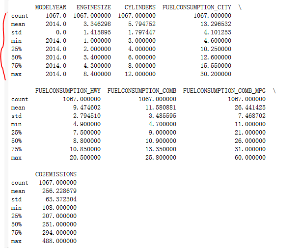
# summarize the data
print(df.describe())

使用describe函数进行表格的预处理，求出最大最小值，已经分比例的数据。

out：

扫描二维码关注公众号，回复： 1998819 查看本文章

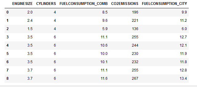
进行表格的重新组合，提取出我们关心的数据类型。

out：

cdf = df[['ENGINESIZE','CYLINDERS','FUELCONSUMPTION_COMB','CO2EMISSIONS','FUELCONSUMPTION_CITY']]
cdf.head(9)

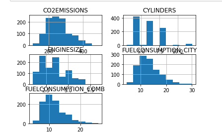
每一列数据可生成hist（直方图）

viz = cdf[['CYLINDERS','ENGINESIZE','CO2EMISSIONS','FUELCONSUMPTION_COMB','FUELCONSUMPTION_CITY']]
viz.hist()
plt.show()

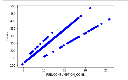
使用scatter生成散列图，定义散列图的参数，颜色

具体使用可参考连接：https://blog.csdn.net/qiu931110/article/details/68130199

plt.scatter(cdf.FUELCONSUMPTION_COMB, cdf.CO2EMISSIONS,  color='blue')
plt.xlabel("FUELCONSUMPTION_COMB")
plt.ylabel("Emission")
plt.show()

选择表中len长度小于8的数据，创建训练集合测试集，并生成散列图

Creating train and test dataset

Train/Test Split involves splitting the dataset into training and testing sets respectively, which are mutually exclusive. After which, you train with the training set and test with the testing set. This will provide a more accurate evaluation on out-of-sample accuracy because the testing dataset is not part of the dataset that have been used to train the data. It is more realistic for real world problems.

This means that we know the outcome of each data point in this dataset, making it great to test with! And since this data has not been used to train the model, the model has no knowledge of the outcome of these data points. So, in essence, it is truly an out-of-sample testing.

msk = np.random.rand(len(df)) < 0.8
train = cdf[msk]
test = cdf[~msk]
print(train)
print(test)

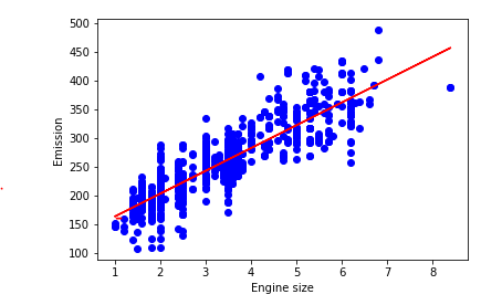
plt.scatter(train.ENGINESIZE, train.CO2EMISSIONS,  color='blue')
plt.xlabel("Engine size")
plt.ylabel("Emission")
plt.show()

Modeling： Using sklearn package to model data.

from sklearn import linear_model
regr = linear_model.LinearRegression()
train_x = np.asanyarray(train[['ENGINESIZE']])
train_y = np.asanyarray(train[['CO2EMISSIONS']])
regr.fit (train_x, train_y)
# The coefficients
print ('Coefficients: ', regr.coef_)
print ('Intercept: ',regr.intercept_)

out：

Coefficients:  [[39.64984954]]
Intercept:  [124.08949291]

As mentioned before, Coefficient and Intercept in the simple linear regression, are the parameters of the fit line. Given that it is a simple linear regression, 
with only 2 parameters, and knowing that the parameters are the intercept and slope of the line, sklearn can estimate them directly from our data. 
Notice that all of the data must be available to traverse and calculate the parameters.

plt.scatter(train.ENGINESIZE, train.CO2EMISSIONS,  color='blue')
plt.plot(train_x, regr.coef_[0][0]*train_x + regr.intercept_[0], '-r')
# 通过斜率和截距画出线性回归曲线
plt.xlabel("Engine size")
plt.ylabel("Emission")

使用sklearn.linear_model.LinearRegression进行线性回归参考以下连接:

https://www.cnblogs.com/magle/p/5881170.html