用户基本分析
library(data.table)
library(dplyr)
library(ggthemr)
library(showtext)
library(cluster)
library(sqldf)
library(NbClust)
library(psych)
library(VGAM)
library(nnet)
library(easyGgplot2)
require(scales)
library(Rwordseg)
library(rJava)
library(tmcn)
ggthemr('fresh')
user <- read.csv('/home/rstudio/work/430_4/user.csv',fileEncoding = 'utf-8')
weibo <- read.csv('/home/rstudio/work/430_4/weibo.csv',fileEncoding = 'utf-8')
user$id <- as.factor(user$id)
weibo$id <- as.factor(weibo$id)
user <- as.data.table(user)
weibo <- as.data.table(weibo)
user <- user[-91,]
modify_weibo <- sqldf::sqldf("select id,name,round(avg(zan),0) as avg_zan,
round(avg(zhuan),0) as avg_zhuanfa ,
round(avg(pinglun),0) as avg_pinglun
from weibo group by id,name")
user_modify_weibo <- left_join( modify_weibo, user,by = c('id','name'))
# 数据整合
user_clu_dt <- select(user_modify_weibo,num_weibo:fans_num,avg_zan:avg_pinglun)
row.names(user_clu_dt) <- user_modify_weibo$name
#dim(user_modify_weibo)
#write.csv(modify_weibo,'weibo1.csv',fileEncoding = 'utf-8')
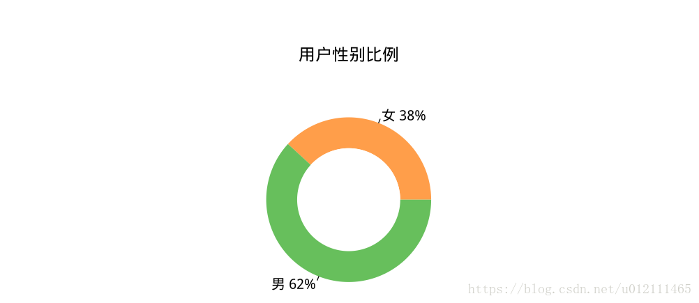
# 性别比例
yy <- table(user$sex)
names(yy) <- c(" 女 38%"," 男 62%")
doughnut <-
function (x, labels = names(x), edges = 200, outer.radius = 0.8,
inner.radius=0.6, clockwise = FALSE,
init.angle = if (clockwise) 90 else 0, density = NULL,
1angle = 45, col = NULL, border = FALSE, lty = NULL,
main = NULL, ...)
{
if (!is.numeric(x) || any(is.na(x) | x < 0))
stop("'x' values must be positive.")
if (is.null(labels))
labels <- as.character(seq_along(x))
else labels <- as.graphicsAnnot(labels)
x <- c(0, cumsum(x)/sum(x))
dx <- diff(x)
nx <- length(dx)
plot.new()
pin <- par("pin")
xlim <- ylim <- c(-1, 1)
if (pin[1L] > pin[2L])
xlim <- (pin[1L]/pin[2L]) * xlim
else ylim <- (pin[2L]/pin[1L]) * ylim
plot.window(xlim, ylim, "", asp = 1)
if (is.null(col))
col <- if (is.null(density))
palette()
else par("fg")
col <- rep(col, length.out = nx)
border <- rep(border, length.out = nx)
lty <- rep(lty, length.out = nx)
angle <- rep(angle, length.out = nx)
density <- rep(density, length.out = nx)
twopi <- if (clockwise)
-2 * pi
else 2 * pi
t2xy <- function(t, radius) {
t2p <- twopi * t + init.angle * pi/180
list(x = radius * cos(t2p),
y = radius * sin(t2p))
}
for (i in 1L:nx) {
n <- max(2, floor(edges * dx[i]))
P <- t2xy(seq.int(x[i], x[i + 1], length.out = n),
outer.radius)
polygon(c(P$x, 0), c(P$y, 0), density = density[i],
angle = angle[i], border = border[i],
col = col[i], lty = lty[i])
Pout <- t2xy(mean(x[i + 0:1]), outer.radius)
lab <- as.character(labels[i])
if (!is.na(lab) && nzchar(lab)) {
lines(c(1, 1.05) * Pout$x, c(1, 1.05) * Pout$y)
text(1.1 * Pout$x, 1.1 * Pout$y, labels[i],
xpd = TRUE, adj = ifelse(Pout$x < 0, 1, 0),
...)
}
## Add white disc
Pin <- t2xy(seq.int(0, 1, length.out = n*nx),
inner.radius)
2polygon(Pin$x, Pin$y, density = density[i],
angle = angle[i], border = border[i],
col = "white", lty = lty[i])
}
title(main = main, ...)
invisible(NULL)
}
# p001 <- doughnut( yy , labels = names(yy),inner.radius=0.5,
# col=c("#FF9E4A", "#67BF5C"),main = ' 用户性别比例')
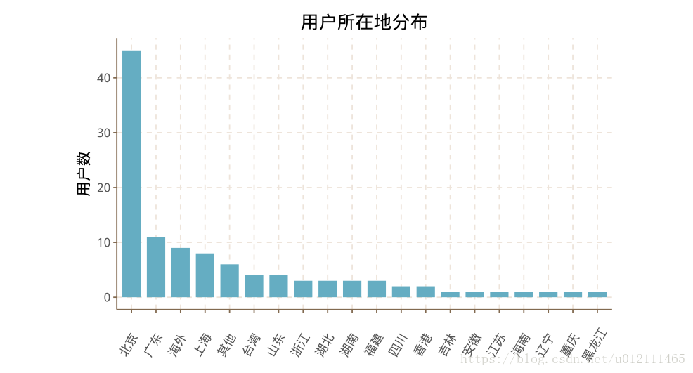
# 用户所在地
place <- as.data.frame(table(user$place))
place <- dplyr::arrange(place,desc(Freq))
place$Var1 <- factor(place$Var1,levels=place$Var1)
p003 <- ggplot(data=place, aes(x= factor(Var1) , y=Freq)) +
geom_col(width = 0.75) +
xlab('') +
ylab(' 用户数') +
labs(title=' 用户所在地分布')+
theme(axis.text.x = element_text(angle = 60, hjust = 0.5, vjust = 0.5),
text = element_text(color = "black", size = 13),
plot.title = element_text(hjust = 0.5))
# 用户微博、关注、粉丝数
WB <- data.frame(Num=user$num_weibo,Name=rep(' 微博',nrow(user)))
GZ <- data.frame(Num=user$guanzhu_num,Name=rep(' 关注',nrow(user)))
FS <- data.frame(Num=user$fans_num,Name=rep(' 粉丝',nrow(user)))
new_dt <- rbind(WB,GZ,FS)
p01 <- ggplot(filter(new_dt,Name==' 微博'), aes(x = Num))+
geom_area(aes(y = ..count..,fill=Name), stat = "bin", alpha = 0.4) +
theme_minimal() +
theme_minimal()+
xlab('') +
ylab(' 用户数') +
labs(title=' 微博数量分布')+
guides(fill=FALSE) +
theme(axis.text.x = element_text(angle = 60, hjust = 0.5, vjust = 0.5),
text = element_text(color = "black", size = 13),
plot.title = element_text(hjust = 0.5))
p02 <- ggplot(filter(new_dt,Name==' 关注'), aes(x = Num))+
geom_area(aes(y = ..count..,fill=Name), stat = "bin", alpha = 0.4) +
theme_minimal() +
theme_minimal()+
xlab('') +
ylab(' 用户数') +
3labs(title=' 关注数量分布')+
guides(fill=FALSE) +
theme(axis.text.x = element_text(angle = 60, hjust = 0.5, vjust = 0.5),
text = element_text(color = "black", size = 13),
plot.title = element_text(hjust = 0.5))
p03 <- ggplot(filter(new_dt,Name==' 粉丝'), aes(x = Num))+
geom_area(aes(y = ..count..,fill=Name), stat = "bin", alpha = 0.4) +
theme_minimal() +
theme_minimal()+
xlab('') +
ylab(' 用户数') +
labs(title=' 粉丝数量分布')+
guides(fill=FALSE) +
theme(axis.text.x = element_text(angle = 60, hjust = 0.5, vjust = 0.5),
text = element_text(color = "black", size = 13),
plot.title = element_text(hjust = 0.5))
# ggplot2.multiplot(p01,p02,p03, cols=3)
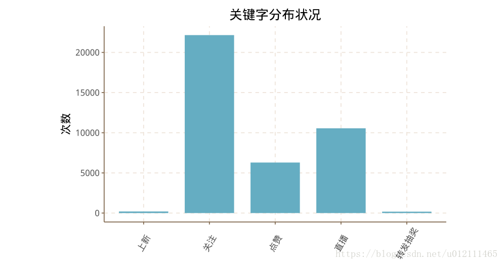
# 关键字
kw <- as.data.frame(table(weibo$key_word))
p4 <- ggplot(data=kw, aes(x= factor(Var1) , y=Freq)) +
geom_col(width = 0.75) +
xlab('') +
ylab(' 次数') +
labs(title=' 关键字分布状况')+
theme(axis.text.x = element_text(angle = 60, hjust = 0.5, vjust = 0.5),
text = element_text(color = "black", size = 13),
plot.title = element_text(hjust = 0.5))
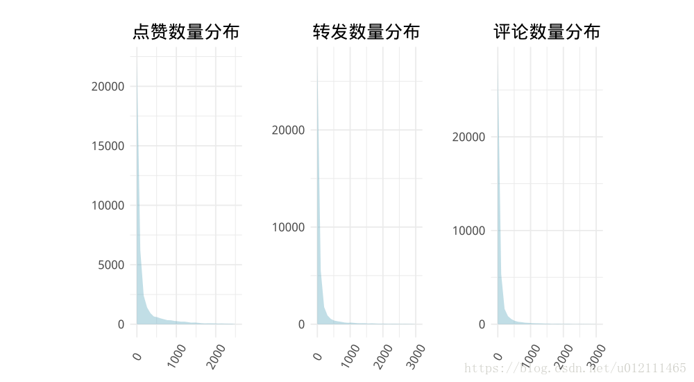
# 点赞、转发、评论数
p1 <- ggplot(filter(weibo,zan<2500), aes(x = zan))+
geom_area(aes(y = ..count..), stat = "bin", alpha = 0.4) +
theme_minimal() +
theme_minimal()+
xlab('') +
ylab('') +
labs(title=' 点赞数量分布')+
guides(fill=FALSE) +
theme(axis.text.x = element_text(angle = 60, hjust = 0.5, vjust = 0.5),
text = element_text(color = "black", size = 13),
plot.title = element_text(hjust = 0.5))
p2 <- ggplot(filter(weibo,zhuan<3000), aes(x = zhuan))+
geom_area(aes(y = ..count..), stat = "bin", alpha = 0.4) +
theme_minimal() +
theme_minimal()+
xlab('') +
4ylab('') +
labs(title=' 转发数量分布')+
guides(fill=FALSE) +
theme(axis.text.x = element_text(angle = 60, hjust = 0.5, vjust = 0.5),
text = element_text(color = "black", size = 13),
plot.title = element_text(hjust = 0.5))
p3 <- ggplot(filter(weibo,pinglun<3000), aes(x = pinglun))+
geom_area(aes(y = ..count..), stat = "bin", alpha = 0.4) +
theme_minimal() +
theme_minimal()+
xlab('') +
ylab('') +
labs(title=' 评论数量分布')+
guides(fill=FALSE) +
theme(axis.text.x = element_text(angle = 60, hjust = 0.5, vjust = 0.5),
text = element_text(color = "black", size = 13),
plot.title = element_text(hjust = 0.5))
# ggplot2.multiplot(p1,p2,p3, cols=3)
# 用户认证身份统计
RZ <- user$renzheng
rz <- ''
for (i in RZ) {
rz <- paste(rz,i)
}
text <- segmentCN(rz)
insertWords(c(" 博主"," 玄幻"," 搞笑"," 脱口秀"," 自媒体"," 央视"," 官方微博",
" 都市报"," 宜家"," 领导力"," 推广人"," 电商"," 萌宠"," 参考消息",
" 曼联"," 育儿"," 魔兽"," 影评人"," 新浪微博"," 官方账号",
" 微博签约"," 微博"))
text <- segmentCN(rz)
#word_sta <- as.data.frame(table(text))
wc <- createWordFreq(unlist(text))
p5 <- wordcloud2(wc,color="random-light",backgroundColor = "grey")- 性别比例
- 用户所在地
- 用户微博、关注、粉丝数
- 关键字
- 微博认证词云图

- 点赞、转发、评论数
聚类分析
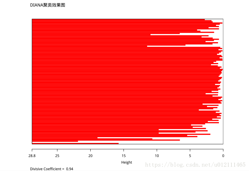
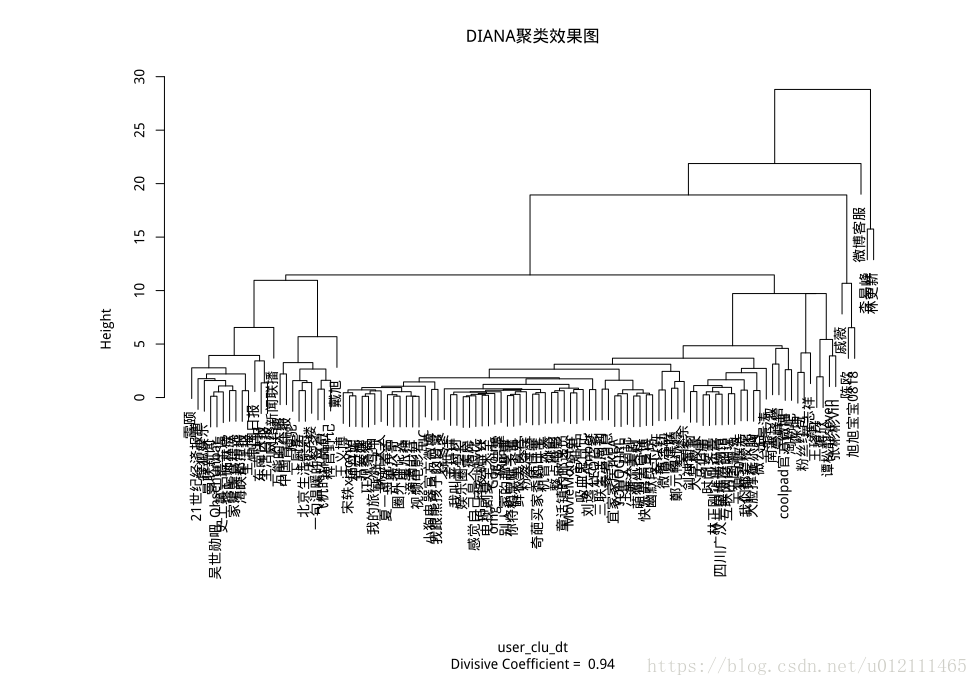
diana_result<- diana(user_clu_dt, metric = "euclidean", stand = TRUE)
plot(diana_result,main="DIANA 聚类效果图")
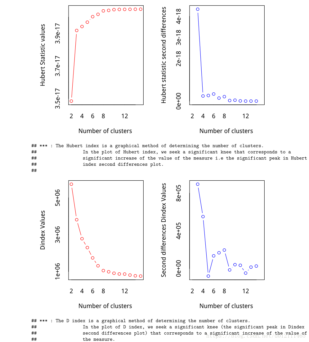
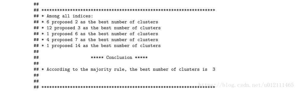
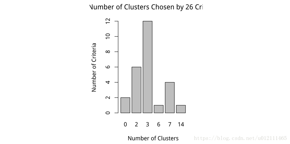
#k-means 确定类数 3
nc <- NbClust(user_clu_dt,min.nc = 2,max.nc = 15,method = "kmeans")
barplot(table(nc$Best.nc[1,]),
xlab="Number of Clusters",
ylab = "Number of Criteria",
main = "Number of Clusters Chosen by 26 Criteria")
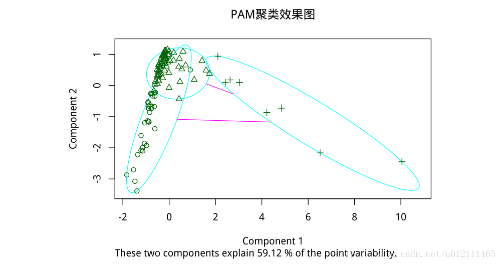
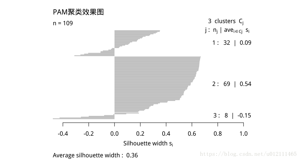
# PAM 算法(聚 3 类)
pamx1=pam(user_clu_dt,k=3, metric = "euclidean", stand = TRUE)
#summary(pamx1)
plot(pamx1,main="PAM 聚类效果图") # 数据集同上
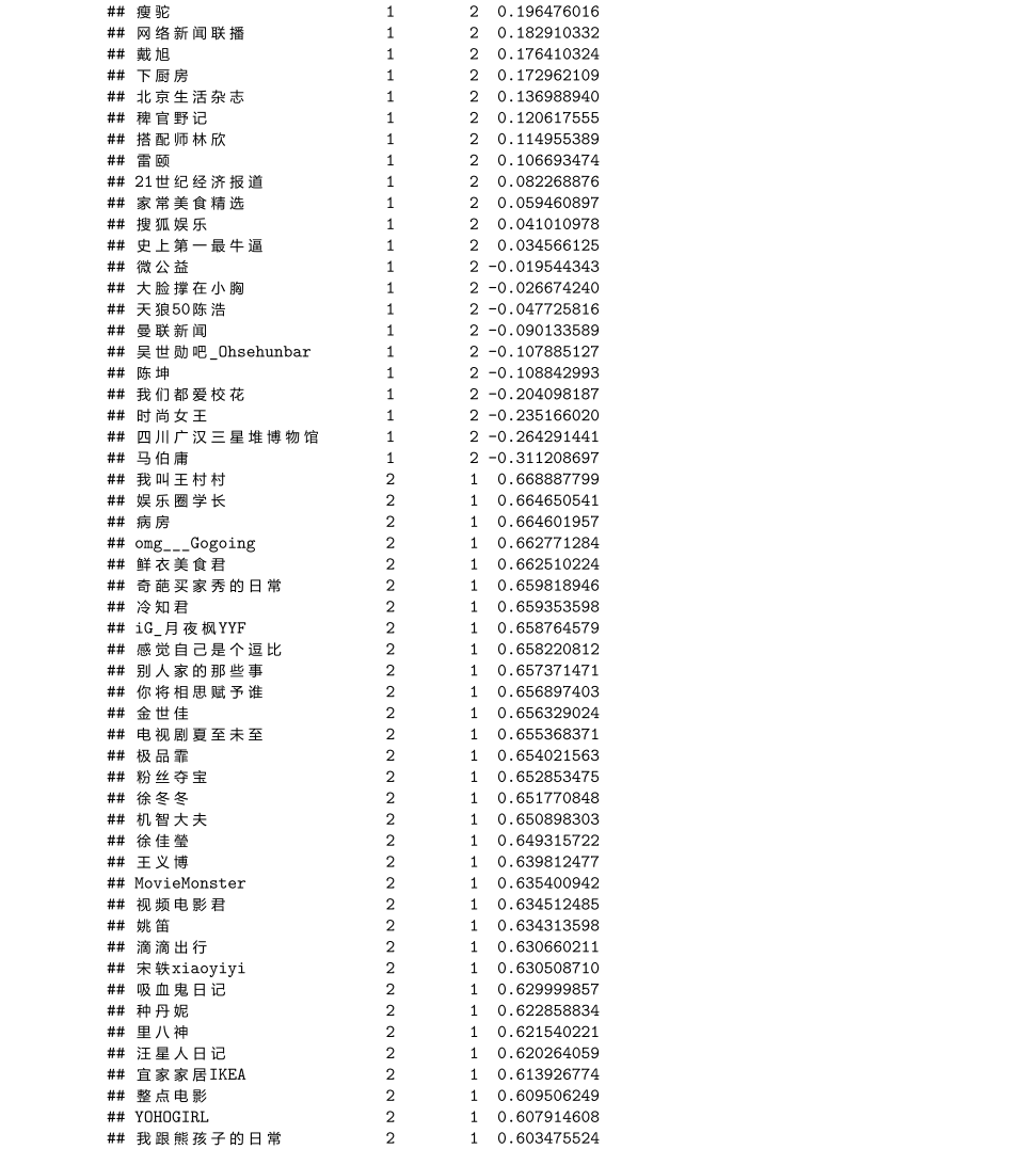
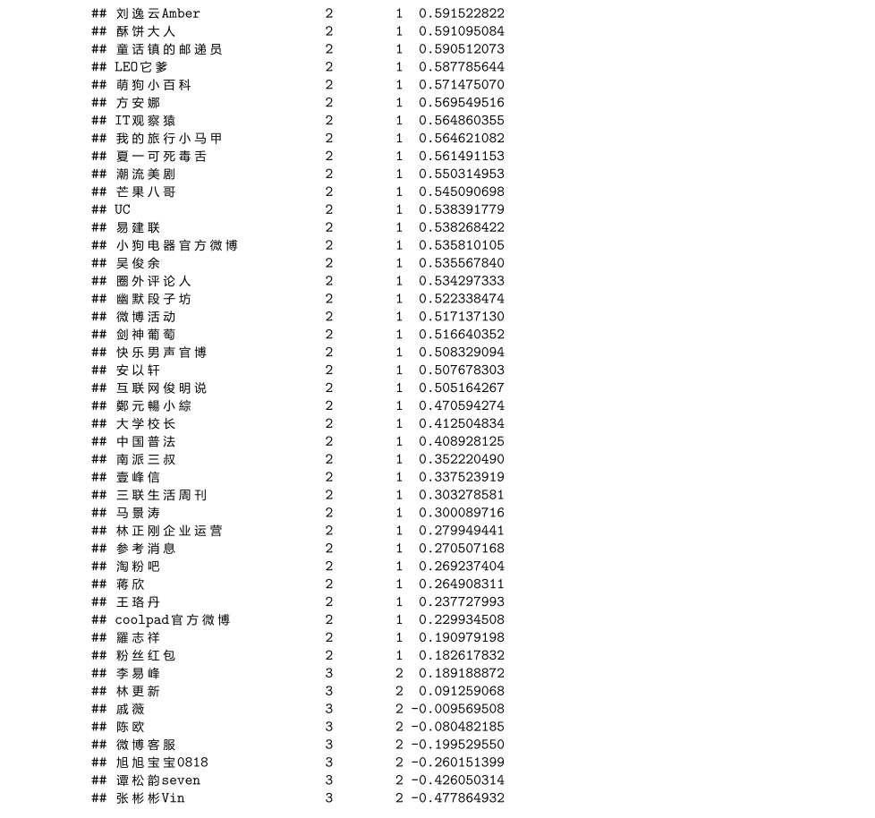
具体聚类划分

Logistic回归
- 构建 logistich 回归数据,结果显示关键字与点赞、评论、转发、用户性别等关系不显著
- 考虑利用 weibo_user 并采用逐步回归进行模型结果输出
结果: - 在此模型中上新作为对照组
- pinglun(评论) 变量增加一个单位,关注 vs 上新的相对危险风险比(the relative risk ratio)是 1.000007,即关注相
对上新来说,评论对关注有影响 - 以此类推,相对上新来说,对关注有影响的变量是性别、转发数、粉丝数、关注数、评论数
- 相对上新来说,对点赞有影响的变量是微博数量、转发数、粉丝数、评论数
- 相对上新来说,对关注有影响的变量是性别、粉丝数、关注数、评论数、赞数
- 相对上新来说,对直播有影响的变量是性别、粉丝数、评论数、评论数、赞数
- 相对上新来说,对直播有影响的变量是性别、粉丝数、评论数、评论数
# 构建模型数据
logit_data <- sqldf::sqldf("select id ,name ,sex ,key_word, avg(num_weibo) as avg_weibo,
avg(guanzhu_num) as avg_wguanzhu,avg(fans_num) as avg_wfan,
avg(zan) as avg_wzan , avg(zhuan) as avg_wzhuan ,
avg(pinglun) as avg_wpinglun from weibo_user
group by id ,name ,sex ,key_word")
# vglm 结果不显著
om <- vglm(key_word ~ factor(sex) + avg_weibo + avg_wguanzhu + avg_wfan + avg_wzan +
avg_wzhuan + avg_wpinglun, data = logit_data,
family = cumulative(parallel = TRUE))
#lrtest(om)
#summary(om)
# 以上不显著,考虑直接利用 weibo_user 表进行建模
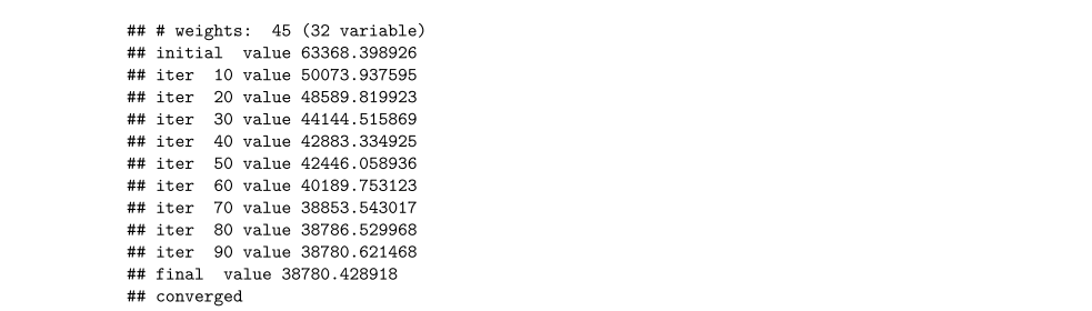
multi_result <- multinom(key_word ~ sex + num_weibo + guanzhu_num + fans_num + zan +
zhuan + pinglun, data = weibo_user)
# summary(multi_result)
# multi_result1<-update(multi_result,~.-1)# 做系数的显著性检验
# multi_result2<-update(multi_result,~.-sex)
# multi_result3<-update(multi_result,~.-num_weibo)
# multi_result4<-update(multi_result,~.-guanzhu_num)
# multi_result5<-update(multi_result,~.-fans_num)
# multi_result6<-update(multi_result,~.-zan)
# multi_result7<-update(multi_result,~.-zhuan)
# multi_result8<-update(multi_result,~.-pinglun)
# anova(multi_result,multi_result1)
# anova(multi_result,multi_result2)
# anova(multi_result,multi_result3)
# anova(multi_result,multi_result4)
# anova(multi_result,multi_result5)
# anova(multi_result,multi_result6)
# anova(multi_result,multi_result7)
# anova(multi_result,multi_result8)
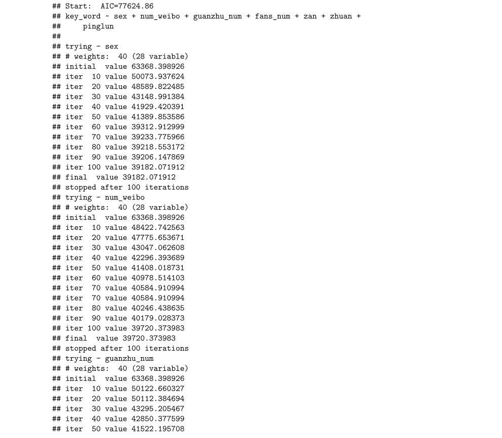
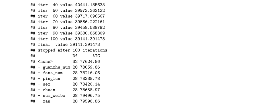
step_result<-step(multi_result) # 逐步回归选元
#summary(step_result)
# 用以解释模型
exp(coef(step_result))