2011年,短链接服务商(URL shortening service)Bitly和美国政府网站USA.gov合作,提供了一份从用户中收集来的匿名数据,这些用户使用了结尾为.gov或.mil的短链接。在2011年,这些数据的动态信息每小时都会保存一次,并可供下载。不过在2017年,这项服务被停掉了。
数据是每小时更新一次,文件中的每一行都用JOSN(JavaScript Object Notation)格式保存。

#coding=gbk

path = r'D:\datasets\example.txt'
line1 = open(path).readline()
print(line1)        #先读取一行数据看看
# { "a": "Mozilla\/5.0 (Windows NT 6.1; WOW64) AppleWebKit\/535.11 (KHTML,----

#使用python的内置的JSON模块,将JSON字符串转换成python字典对象
import json
records = [json.loads(line) for line in open(path)]
print(records[0])       #返回的结果对象records是一个有字典组成的数组
# {'hc': 1331822918, 'u': 'http://www.ncbi.nlm.nih.gov/pubmed/22415991', 'gr': 'MA',
print(records[0]['tz']) # America/New_York 现在可以进行键值对查找 tz表示时区
1. 先使用纯python对时区进行计数
# time_zones = [rec['tz'] for rec in records ] 此处有些tz 是为空的, 执行会报错
time_zones = [rec['tz'] for rec in records if 'tz' in rec]
print(time_zones[5:11]) #可以看到有空数据的存在
# ['America/New_York', 'Europe/Warsaw', '', '', '', 'America/Los_Angeles']

#遍历时区,统计时区出现的数目,保留到字典当中
# def get_counts(sequence):
#     counts = {}
#     for x in sequence:
#         if x in counts:
#             counts[x] += 1
#         else:
#             counts[x] = 1
#     return counts
#这里可以使用python标准库中defaultdict,与上述的代码得到结果是一样的
#可以使代码变得更简洁
from collections import defaultdict
def get_counts(sequence):
    counts = defaultdict(int)
    for x in sequence:
        counts[x] += 1
    return counts
counts = get_counts(time_zones)
print(counts['Europe/Warsaw'])  # 16

# 获取前10 位的时区及其计数值
# dict = {"a" : "apple", "b" : "banana", "c" : "grape", "d" : "orange"}
# it = dict.get('a') #此种方法查询,如果找不到的话, 不会报错
# print(it)   # None
# l = []
# for key, value in dict.items():
#     l.append([key,value])
# print(l)
def top_counts(count_dict, n=10):
    value_key_pairs = [(count, tz) for tz, count in count_dict.items()]
    value_key_pairs.sort()  # 依据数量进行排序
    return value_key_pairs[-n:]
print(top_counts(counts, n=3))  #输出前3 项时区最多的地方及数量
# [(400, 'America/Chicago'), (521, ''), (1251, 'America/New_York')]

#使用python 标准库里的 collections.Counter 类,
from collections import Counter
counts = Counter(time_zones)
most3 = counts.most_common(3)
print(most3)
# [('America/New_York', 1251), ('', 521), ('America/Chicago', 400)]
2. 使用pandas 对时区进行计数及其他可视化操作
import pandas as pd
import numpy as np
frame = pd.DataFrame(records)
print(frame.info())
#对时区的统计, pandas只需要一行代码即可, pandas可谓强大
tz_counts = frame['tz'].value_counts()
print(tz_counts[:5])
# America/New_York       1251
#                         521
# America/Chicago         400
# America/Los_Angeles     382
# America/Denver          191
# Name: tz, dtype: int64

#使用fillna函数替代缺失值,而空字符可以使用 布尔类型数组索引
clean_tz = frame['tz'].fillna('Missing')
print(clean_tz[5:11])   # 还是为空值
clean_tz[clean_tz == ''] ='Unknown'
tz_counts = clean_tz.value_counts()
print(tz_counts[:5])
# America/New_York       1251
# Unknown                 521
# America/Chicago         400
# America/Los_Angeles     382
# America/Denver          191
# Name: tz, dtype: int64
%matplotlib inline
tz_counts[:10].plot(kind='barh', rot=0)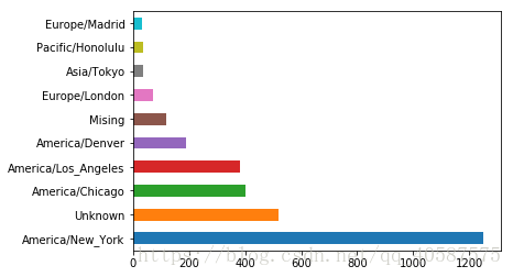
import seaborn as sns
subset = tz_counts[:10]
sns.barplot(y=subset.index, x = subset.values)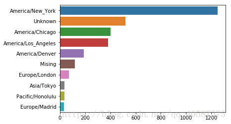
#可以把字符串的第一节分离出来, 大致是对应其浏览器
results = pd.Series([x.split()[0] for x in frame.a.dropna()]) #[0] 是获得第一项数据
print(results[:5])
# 0 Mozilla/5.0 #火狐浏览器
# 1 GoogleMaps/RochesterNY
# 2 Mozilla/4.0
# 3 Mozilla/5.0
# 4 Mozilla/5.0
# dtype: object
print(results.value_counts()[:5])
# Mozilla/5.0 2594
# Mozilla/4.0 601
# GoogleMaps/RochesterNY 121
# Opera/9.80 34
# TEST_INTERNET_AGENT 24
# dtype: int64
#接下来, 按Windows 和非Windows 用户对时区进行分解,由于有agent的缺失,先将其移除
cframe = frame[frame.a.notnull()]
# print(cframe.head())
#新增一行特征属性,将有Windows字符的数据认为是 微软的操作系统
cframe['os'] = np.where(cframe.a.str.contains('Windows'), 'Windows', 'Not Windows')
print(cframe.os[:5])
# 0 Windows
# 1 Not Windows
# 2 Windows
# 3 Not Windows
# 4 Windows
# Name: os, dtype: object
#根据时区和操作系统进行分组
by_tz_os = cframe.groupby(['tz', 'os'])
print(by_tz_os.size()[:5]) #打印出前5 行, size()对分组结果进行计数, 类似于value_counts函数
# tz os
# Not Windows 245
# Windows 276
# Africa/Cairo Windows 3
# Africa/Casablanca Windows 1
# Africa/Ceuta Windows 2
# dtype: int64
agg_counts = by_tz_os.size().unstack().fillna(0) #使用unstack 对计数结果重塑成一个表格
print(agg_counts[:5])
# os Not Windows Windows
# tz
# 245.0 276.0
# Africa/Cairo 0.0 3.0
# Africa/Casablanca 0.0 1.0
# Africa/Ceuta 0.0 2.0
# Africa/Johannesburg 0.0 1.0
#根据agg_counts中的行数构造一个简洁的索引数组
indexer = agg_counts.sum(1).argsort()
print(indexer[:5])
# tz
# 24
# Africa/Cairo 20
# Africa/Casablanca 21
# Africa/Ceuta 92
# Africa/Johannesburg 87
# dtype: int64
#使用take 按照这个顺序截取最后10 行
count_subset = agg_counts.take(indexer)[-10:]
print(count_subset)
# os Not Windows Windows
# tz
# America/Denver 132.0 59.0
# America/Los_Angeles 130.0 252.0
# America/Chicago 115.0 285.0
# 245.0 276.0
# America/New_York 339.0 912.0
count_subset = count_subset.stack()
count_subset.name = 'total'
count_subset = count_subset.reset_index() # 重新建立索引,不把地址 作为索引
print(count_subset[:5])
# tz os total
# 0 America/Sao_Paulo Not Windows 13.0
# 1 America/Sao_Paulo Windows 20.0
# 2 Europe/Madrid Not Windows 16.0
# 3 Europe/Madrid Windows 19.0
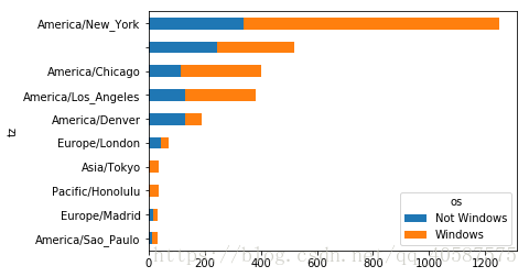
# 4 Pacific/Honolulu Not Windows 0.0sns.barplot(x = 'total',y='tz', hue='os',data= count_subset)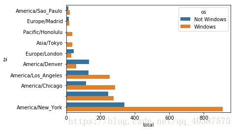
由于不能很好地看出Windows用户与其他用户的区别, 所以对各行进行归一化处理
def norm_total(group):
    group['normed_total'] = group.total / group.total.sum()
    return group
def norm_total(group):
    group['normed_total'] = group.total / group.total.sum()
    return group
In [57]:

results = count_subset.groupby('tz').apply(norm_total)
sns.barplot(x='normed_total', y= 'tz', hue='os', data =results)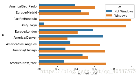
count_subset = agg_counts.take(indexer)[-10:]
count_subset

Out[58]:
os	Not Windows	Windows
tz
America/Sao_Paulo	13.0	20.0
Europe/Madrid	16.0	19.0
Pacific/Honolulu	0.0	36.0
Asia/Tokyo	2.0	35.0
Europe/London	43.0	31.0
America/Denver	132.0	59.0
America/Los_Angeles	130.0	252.0
America/Chicago	115.0	285.0
245.0	276.0
America/New_York	339.0	912.0
count_subset.plot(kind='barh', stacked=True)#stacked 为堆积条形图
normed_subset = count_subset.div(count_subset.sum(1), axis=0)
normed_subset.plot(kind='barh', stacked = True)
参考:《利用Python进行数据分析》