参数设置

α：

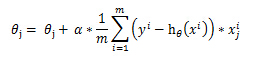
梯度上升算法迭代时候权重更新公式中包含 α ：

这里写图片描述
http://blog.csdn.net/lu597203933/article/details/38468303
为了更好理解 α和最大迭代次数的作用，给出Python版的函数计算过程。

# 梯度上升算法-计算回归系数  
# 每个回归系数初始化为1
# 重复R次：
#    计算整个数据集的梯度
#    使用α*梯度更新回归系数的向量
#    返回回归系数
def gradAscent(dataMatIn, classLabels,alpha=0.001,maxCycles = 500):  
    dataMatrix = mat(dataMatIn)     #转换为numpy数据类型  
    labelMat = mat(classLabels).transpose()  
    m,n = shape(dataMatrix)      
    maxCycles = 500  
    weights = ones((n,1))  
    for k in range(maxCycles):  
        h = sigmoid(dataMatrix*weights)  
        error = (labelMat - h)  
        #计算真实类别与预测类别的差值，按照该差值的方向调整回归系数
        weights = weights + alpha* dataMatrix.transpose() * error  
    return weights

λ

λ，正则化参数（泛化能力），加正则化的前提是特征值要进行归一化。

在实际应该过程中，为了增强模型的泛化能力，防止我们训练的模型过拟合，特别是对于大量的稀疏特征，模型复杂度比较高，需要进行降维，我们需要保证在训练误差最小化的基础上，通过加上正则化项减小模型复杂度。在逻辑回归中，有L1、L2进行正则化。>
损失函数如下：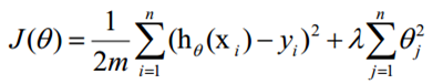

http://www.bkjia.com/yjs/996300.html
在损失函数里加入一个正则化项，正则化项就是权重的L1或者L2范数乘以一个λ，用来控制损失函数和正则化项的比重，直观的理解，首先防止过拟合的目的就是防止最后训练出来的模型过分的依赖某一个特征，当最小化损失函数的时候，某一维度很大，拟合出来的函数值与真实的值之间的差距很小，通过正则化可以使整体的cost变大，从而避免了过分依赖某一维度的结果。当然加正则化的前提是特征值要进行归一化。

threshold

threshold变量用来控制分类的阈值，默认值为0.5。表示如果预测值小于threshold则为分类0.0，否则为1.0。

在Spark Java中
ElasticNetParam ： α ；RegParam ：λ。

LogisticRegression lr=new LogisticRegression()
                .setMaxIter(10)
                .setRegParam(0.3)
                .setElasticNetParam(0.2)                
                .setThreshold(0.5);

分类效果评估

参考：http://www.cnblogs.com/tovin/p/3816289.html
http://blog.sina.com.cn/s/blog_900690c60101czyo.html
http://blog.chinaunix.net/uid-446337-id-94448.html
http://blog.csdn.net/abcjennifer/article/details/7834256

混淆矩阵（Confusion matrix）：
考虑一个二分问题，即将实例分成正类（positive）或负类（negative）。对一个二分问题来说，会出现四种情况。如果一个实例是正类并且也被预测成正类，即为真正类（True positive）,如果实例是负类被预测成正类，称之为假正类（False positive）。相应地，如果实例是负类被预测成负类，称之为真负类（True negative）,正类被预测成负类则为假负类（false negative）。
TP：正确肯定的数目；
FN：漏报，没有正确找到的匹配的数目；
FP：误报，给出的匹配是不正确的；
TN：正确拒绝的非匹配对数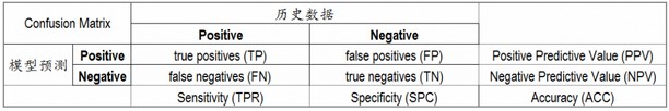
这里写图片描述
精确率，precision = TP / (TP + FP)
模型判为正的所有样本中有多少是真正的正样本
召回率，recall = TP / (TP + FN)
准确率，accuracy = (TP + TN) / (TP + FP + TN + FN)
反映了分类器统对整个样本的判定能力——能将正的判定为正，负的判定为负
如何在precision和Recall中权衡？
F1 Score = P*R/2(P+R)，其中P和R分别为 precision 和 recall
在precision与recall都要求高的情况下，可以用F1 Score来衡量

为什么会有这么多指标呢？
这是因为模式分类和机器学习的需要。判断一个分类器对所用样本的分类能力或者在不同的应用场合时，需要有不同的指标。当总共有个100 个样本（P+N=100）时，假如只有一个正例（P=1），那么只考虑精确度的话，不需要进行任何模型的训练，直接将所有测试样本判为正例，那么 A 能达到 99%，非常高了，但这并没有反映出模型真正的能力。另外在统计信号分析中，对不同类的判断结果的错误的惩罚是不一样的。举例而言，雷达收到100个来袭导弹的信号，其中只有 3个是真正的导弹信号，其余 97 个是敌方模拟的导弹信号。假如系统判断 98 个（97 个模拟信号加一个真正的导弹信号）信号都是模拟信号，那么Accuracy=98%，很高了，剩下两个是导弹信号，被截掉，这时Recall=2/3=66.67%，Precision=2/2=100%，Precision也很高。但剩下的那颗导弹就会造成灾害。

ROC曲线和AUC
有时候我们需要在精确率与召回率间进行权衡，
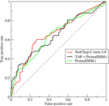
调整分类器threshold取值，以FPR（假正率False-positive rate）为横坐标，TPR（True-positive rate）为纵坐标做ROC曲线；
Area Under roc Curve(AUC)：处于ROC curve下方的那部分面积的大小通常，AUC的值介于0.5到1.0之间，较大的AUC代表了较好的性能；
精确率和召回率是互相影响的，理想情况下肯定是做到两者都高，但是一般情况下准精确率、召回率就低，召回率低、精确率高，当然如果两者都低，那是什么地方出问题了
这里写图片描述

Spark 2.0分类评估

//获得回归模型训练的Summary
LogisticRegressionTrainingSummary trainingSummary = lrModel.summary();

// Obtain the loss per iteration.
//每次迭代的损失，一般会逐渐减小
double[] objectiveHistory = trainingSummary.objectiveHistory();
for (double lossPerIteration : objectiveHistory) {
  System.out.println(lossPerIteration);
}

// Obtain the metrics useful to judge performance on test data.
// We cast the summary to a BinaryLogisticRegressionSummary since the problem is a binary
// classification problem.
//强制类型转换为二类LR的Summary，然后就可以用混淆矩阵,ROC等评估方法了。Spark2.0还无法针对多类
BinaryLogisticRegressionSummary binarySummary =
  (BinaryLogisticRegressionSummary) trainingSummary;

// Obtain the receiver-operating characteristic as a dataframe and areaUnderROC.
Dataset<Row> roc = binarySummary.roc();//获得ROC
roc.show();//显示ROC数据表，可以用这个数据自己画ROC曲线
roc.select("FPR").show();
System.out.println(binarySummary.areaUnderROC());//AUC

// Get the threshold corresponding to the maximum F-Measure and rerun LogisticRegression with
// this selected threshold.
//不同的阈值，计算不同的F1，然后通过最大的F1找出并重设模型的最佳阈值。
Dataset<Row> fMeasure = binarySummary.fMeasureByThreshold();
double maxFMeasure = fMeasure.select(functions.max("F-Measure")).head().getDouble(0);//获得最大的F1值
double bestThreshold = fMeasure.where(fMeasure.col("F-Measure").equalTo(maxFMeasure))
  .select("threshold").head().getDouble(0);//找出最大F1值对应的阈值（最佳阈值）
lrModel.setThreshold(bestThreshold);//并将模型的Threshold设置为选择出来的最佳分类阈值

Logistic回归完整的代码
http://spark.apache.org/docs/latest/ml-classification-regression.html

package my.spark.ml.practice.classification;

import org.apache.log4j.Level;
import org.apache.log4j.Logger;
import org.apache.spark.ml.classification.BinaryLogisticRegressionTrainingSummary;
import org.apache.spark.ml.classification.LogisticRegression;
import org.apache.spark.ml.classification.LogisticRegressionModel;
import org.apache.spark.ml.classification.LogisticRegressionTrainingSummary;
import org.apache.spark.sql.Dataset;
import org.apache.spark.sql.Row;
import org.apache.spark.sql.SparkSession;
import org.apache.spark.sql.functions;


public class myLogisticRegression {

    public static void main(String[] args) {
        SparkSession spark=SparkSession
                .builder()
                .appName("LR")
                .master("local[4]")
                .config("spark.sql.warehouse.dir","file///:G:/Projects/Java/Spark/spark-warehouse" )
                .getOrCreate();
        String path="G:/Projects/CgyWin64/home/pengjy3/softwate/spark-2.0.0-bin-hadoop2.6/"
                + "data/mllib/sample_libsvm_data.txt";

        //屏蔽日志
        Logger.getLogger("org.apache.spark").setLevel(Level.WARN);
        Logger.getLogger("org.eclipse.jetty.server").setLevel(Level.OFF);       

        //Load trainning data
        Dataset<Row> trainning_dataFrame=spark.read().format("libsvm").load(path);      


        LogisticRegression lr=new LogisticRegression()
                .setMaxIter(10)
                .setRegParam(0.3)
                .setElasticNetParam(0.2)                
                .setThreshold(0.5);

        //fit the model
        LogisticRegressionModel lrModel=lr.fit(trainning_dataFrame);

        //print the coefficients and intercept for logistic regression
        System.out.println
        ("Coefficient:"+lrModel.coefficients()+"Itercept"+lrModel.intercept());

        //Extract the summary from the returned LogisticRegressionModel
        LogisticRegressionTrainingSummary summary=lrModel.summary();

        //Obtain the loss per iteration.
        double[] objectiveHistory=summary.objectiveHistory();
        for(double lossPerIteration:objectiveHistory){
            System.out.println(lossPerIteration);
        }
        // Obtain the metrics useful to judge performance on test data.
        // We cast the summary to a BinaryLogisticRegressionSummary since the problem is a binary
        // classification problem.
        BinaryLogisticRegressionTrainingSummary binarySummary=
                (BinaryLogisticRegressionTrainingSummary)summary;
        //Obtain the receiver-operating characteristic as a dataframe and areaUnderROC.
        Dataset<Row> roc=binarySummary.roc();
        roc.show((int) roc.count());//显示全部的信息，roc.show()默认只显示20行
        roc.select("FPR").show();
        System.out.println(binarySummary.areaUnderROC());

        // Get the threshold corresponding to the maximum F-Measure and rerun LogisticRegression with
        // this selected threshold.
        Dataset<Row> fMeasure = binarySummary.fMeasureByThreshold();
        double maxFMeasure = fMeasure.select(functions.max("F-Measure")).head().getDouble(0);
        double bestThreshold = fMeasure.where(fMeasure.col("F-Measure").equalTo(maxFMeasure))
          .select("threshold").head().getDouble(0);
        lrModel.setThreshold(bestThreshold);            
    }

}

BinaryClassificationEvaluator

除了上述Logistic回归结果评估方法，在Spark2.0中，二分问题结果评估用BinaryClassificationEvaluator。
参数：
（1）labelCol: label column name (default: label, current: label)
（2）metricName: metric name in evaluation (areaUnderROC|areaUnderPR) (default: areaUnderROC)
看来是没有其它的评估方法
（3）rawPredictionCol: raw prediction (a.k.a. confidence) column name (default: rawPrediction, current: prediction)：注意名字不是PredictionCol，
只有这三个参数可以设置！
自定义accuracy

//自定义计算accuracy，
        Dataset<Row> predictDF=naiveBayesModel.transform(test);    

        double total=(double) predictDF.count();
        Encoder<Double> doubleEncoder=Encoders.DOUBLE();        
        Dataset<Double> accuracyDF=predictDF.map(new MapFunction<Row,Double>() {            
            @Override
            public Double call(Row row) throws Exception {
                if((double)row.get(0)==(double)row.get(6)){return 1.0;}
                else {return 0.0;}
            }
        }, doubleEncoder);
        accuracyDF.createOrReplaceTempView("view");
        double correct=(double) spark.sql("SELECT value FROM view WHERE value=1.0").count();
        System.out.println("accuracy "+(correct/total));

Scikit

关键代码分析

#For L1 penalization sklearn.svm.l1_min_c allows to calculate the
#lower bound for C in order to get a non “null” (all feature 
#weights to zero) model. 
#计算一个C的下限值，然后放大到一个区间内。
cs = l1_min_c(X, y, loss='log') * np.logspace(0, 3)

print("l1_min_c=%.4f"%l1_min_c(X, y, loss='log'))
#输出结果:l1_min_c=0.0143

clf = linear_model.LogisticRegression(C=1.0, penalty='l1', tol=1e-6)
coefs_ = []
for c in cs:#循环不同的C
    clf.set_params(C=c)#重新设置C
    clf.fit(X, y)#重新计算
    coefs_.append(clf.coef_.ravel().copy())#获得系数
    print("score %.4f" % clf.score(X, y))#计算分类的score
coefs_ = np.array(coefs_)#将系数转为np.array
plt.plot(np.log10(cs), coefs_)#作图 log(C)vs Coefs

关键参数C，penalty
penalty选择’l1’，’l2’
C：large values of C give more freedom to the model. Conversely, smaller values of C constrain the model more（C，也控制着模型的泛化能力，与前面Spark中所说的RegParam -λ作用类似）

Scikit中的LR可以完成多类（one-vs-rest）的分类，L1或L2正则化。

This implementation can fit a multiclass (one-vs-rest) logistic regression with optional L2 or L1 regularization.
binary class L2 penalized logistic regression minimizes the following cost function：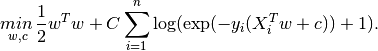

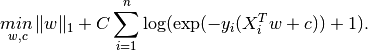
L1 regularized logistic regression solves the following optimization problem

不同情形算法选择：
Small dataset or L1 penalty —-> “liblinear”
Multinomial loss —–> “lbfgs” or newton-cg”
Large dataset —–> “sag”

“Sag”：随机平均梯度下降算法，Stochastic Average Gradient descent ，在大数据集上通常比其它算法要快。

It does not handle “multinomial” case, and is limited to L2-penalized
models, yet it is often faster than other solvers for large datasets,
when both the number of samples and the number of features are large.
Stochastic gradient descent is a simple yet very efficient approach to fit linear models. It is particularly useful when the number of samples (and the number of features) is very large.

完整的代码如下：

print(__doc__)

# Author: Alexandre Gramfort <[email protected]>
# License: BSD 3 clause

from datetime import datetime
import numpy as np
import matplotlib.pyplot as plt

from sklearn import linear_model
from sklearn import datasets
from sklearn.svm import l1_min_c

iris = datasets.load_iris()
X = iris.data
y = iris.target

X = X[y != 2]
y = y[y != 2]

X -= np.mean(X, 0)

###############################################################################
# Demo path functions

cs = l1_min_c(X, y, loss='log') * np.logspace(0, 3)

print("Computing regularization path ...")
start = datetime.now()
clf = linear_model.LogisticRegression(C=1.0, penalty='l1', tol=1e-6)
coefs_ = []
for c in cs:
    clf.set_params(C=c)
    clf.fit(X, y)
    coefs_.append(clf.coef_.ravel().copy())
print("This took ", datetime.now() - start)

coefs_ = np.array(coefs_) #50*4维矩阵
plt.plot(np.log10(cs), coefs_)
ymin, ymax = plt.ylim()
plt.xlabel('log(C)')
plt.ylabel('Coefficients')
plt.title('Logistic Regression Path')
plt.axis('tight')
plt.show()

Spark2.0机器学习系列之2：Logistic回归及Binary分类（二分问题）结果评估