目录
2.2 滑窗交叉验证(SildingWindowForecastCV)
1. pmdarima实现单变量时间序列预测
Pmdarima是以statsmodel和autoarima为基础、封装研发出的Python时序分析库、也是现在市面上封装程度最高、代码最为简洁的时序预测库之一。Pmdarima由sklearn团队开发,沿袭了sklearn库的代码习惯、并保留了一切接入sklearn的接口,是非常方便机器学习学习者学习的工具。该库包括了以R语言为基础的autoarima所有的功能,并且能够处理平稳性、季节性、周期性等问题,可以执行差分、交叉验证等运算,以及内容丰富的官方说明文档。以下是使用Pmdarima实现一个简单预测的过程:
import pmdarima as pm
from pmdarima import model_selection
import numpy as np
import pandas as pd
import matplotlib.pyplot as plt
from sklearn.metrics import mean_squared_error
import warnings
warnings.filterwarnings("ignore")

data = pm.datasets.load_wineind()
len(data) #176

fig=plt.figure(figsize=(16,5))
plt.plot(range(data.shape[0]),data)
plt.grid()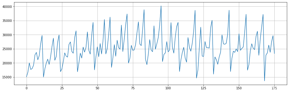
#使用pm分割数据,遵循时序规则,不会打乱时间顺序
train, test = model_selection.train_test_split(data, train_size=152)
#自动化建模,只支持SARIMAX混合模型,不支持VARMAX系列模型
arima = pm.auto_arima(train, trace=True, #训练数据,是否打印训练过程?
                      error_action='ignore', suppress_warnings=True, #无视警告和错误
                      maxiter=5, #允许的最大迭代次数
                      seasonal=True, m=12 #是否使用季节性因子?如果使用的话,多步预测的步数是多少?
                     )
Performing stepwise search to minimize aic ARIMA(2,1,2)(1,0,1)[12] intercept : AIC=2955.247, Time=0.46 sec ARIMA(0,1,0)(0,0,0)[12] intercept : AIC=3090.160, Time=0.02 sec ARIMA(1,1,0)(1,0,0)[12] intercept : AIC=2993.480, Time=0.08 sec ARIMA(0,1,1)(0,0,1)[12] intercept : AIC=2985.395, Time=0.09 sec ARIMA(0,1,0)(0,0,0)[12] : AIC=3088.177, Time=0.02 sec ARIMA(2,1,2)(0,0,1)[12] intercept : AIC=2978.426, Time=0.16 sec ARIMA(2,1,2)(1,0,0)[12] intercept : AIC=2954.744, Time=0.18 sec ARIMA(2,1,2)(0,0,0)[12] intercept : AIC=3025.510, Time=0.10 sec ARIMA(2,1,2)(2,0,0)[12] intercept : AIC=2954.236, Time=0.49 sec ARIMA(2,1,2)(2,0,1)[12] intercept : AIC=2958.264, Time=0.49 sec ARIMA(1,1,2)(2,0,0)[12] intercept : AIC=2964.588, Time=0.38 sec ARIMA(2,1,1)(2,0,0)[12] intercept : AIC=2950.034, Time=0.53 sec ARIMA(2,1,1)(1,0,0)[12] intercept : AIC=2950.338, Time=0.24 sec ARIMA(2,1,1)(2,0,1)[12] intercept : AIC=2953.291, Time=0.45 sec ARIMA(2,1,1)(1,0,1)[12] intercept : AIC=2951.569, Time=0.21 sec ARIMA(1,1,1)(2,0,0)[12] intercept : AIC=2958.953, Time=0.32 sec ARIMA(2,1,0)(2,0,0)[12] intercept : AIC=2966.286, Time=0.35 sec ARIMA(3,1,1)(2,0,0)[12] intercept : AIC=2951.433, Time=0.50 sec ARIMA(1,1,0)(2,0,0)[12] intercept : AIC=2993.310, Time=0.39 sec ARIMA(3,1,0)(2,0,0)[12] intercept : AIC=2952.990, Time=0.47 sec ARIMA(3,1,2)(2,0,0)[12] intercept : AIC=2953.842, Time=0.58 sec ARIMA(2,1,1)(2,0,0)[12] : AIC=2946.471, Time=0.45 sec ARIMA(2,1,1)(1,0,0)[12] : AIC=2947.171, Time=0.17 sec ARIMA(2,1,1)(2,0,1)[12] : AIC=2948.216, Time=0.42 sec ARIMA(2,1,1)(1,0,1)[12] : AIC=2946.151, Time=0.29 sec ARIMA(2,1,1)(0,0,1)[12] : AIC=2971.736, Time=0.14 sec ARIMA(2,1,1)(1,0,2)[12] : AIC=2948.085, Time=0.50 sec ARIMA(2,1,1)(0,0,0)[12] : AIC=3019.258, Time=0.06 sec ARIMA(2,1,1)(0,0,2)[12] : AIC=2959.185, Time=0.36 sec ARIMA(2,1,1)(2,0,2)[12] : AIC=2950.098, Time=0.52 sec ARIMA(1,1,1)(1,0,1)[12] : AIC=2953.184, Time=0.14 sec ARIMA(2,1,0)(1,0,1)[12] : AIC=2964.069, Time=0.14 sec ARIMA(3,1,1)(1,0,1)[12] : AIC=2949.076, Time=0.16 sec ARIMA(2,1,2)(1,0,1)[12] : AIC=2951.826, Time=0.16 sec ARIMA(1,1,0)(1,0,1)[12] : AIC=2991.086, Time=0.09 sec ARIMA(1,1,2)(1,0,1)[12] : AIC=2960.917, Time=0.14 sec ARIMA(3,1,0)(1,0,1)[12] : AIC=2950.719, Time=0.13 sec ARIMA(3,1,2)(1,0,1)[12] : AIC=2952.019, Time=0.17 sec Best model: ARIMA(2,1,1)(1,0,1)[12] Total fit time: 11.698 seconds
#预测
preds = arima.predict(n_periods=test.shape[0])
preds #按照测试集的日期进行预测
array([25809.09822027, 27111.50500611, 30145.84346715, 35069.09860267,
19044.09098919, 22734.07766136, 24370.14476344, 24468.4989244 ,
24661.71940304, 24465.6250753 , 29285.02123954, 25607.32326197,
26131.79439226, 26937.20321329, 29632.82588046, 33904.51565498,
20207.31393733, 23342.10936251, 24741.41755828, 24828.6385991 ,
24993.22466868, 24825.14042152, 28939.23990247, 25799.92370898])
fig=plt.figure(figsize=(16,5))
plt.plot(range(test.shape[0]),test)
plt.plot(range(test.shape[0]),preds)
plt.grid()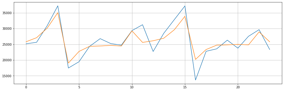
模型评估指标可共有sklearn的评估指标,也可调用特定的时序指标AIC:
np.sqrt(mean_squared_error(test, preds))2550.8826581401277
arima.aic()2946.1506587436375
arima.summary()
枚举式搜索合适的参数,从效率角度来说远远超过statsmodel,遗憾的是,从上述代码不难看出pmdarima的代码思路是更最近机器学习而不是统计学的,因此pmd.auto arima跑出的结果往往无法满足统计学上的各类检验要求,因此泛化能力无法被保证。同时也很容易发现,由于数据集分割的缘故,autoarima选择出的最佳模型可能无法被复现,例如我们使用autoarima选择出的最佳模型建立单模:
model=pm.ARIMA(order=(2,1,1),seasonal_order=(1,0,1,12),max_iter=500)
model.fit(train)

fig=plt.figure(figsize=(16,5))
plt.plot(range(test.shape[0]),test)
plt.plot(range(test.shape[0]),model.predict(n_periods=test.shape[0]))
plt.grid()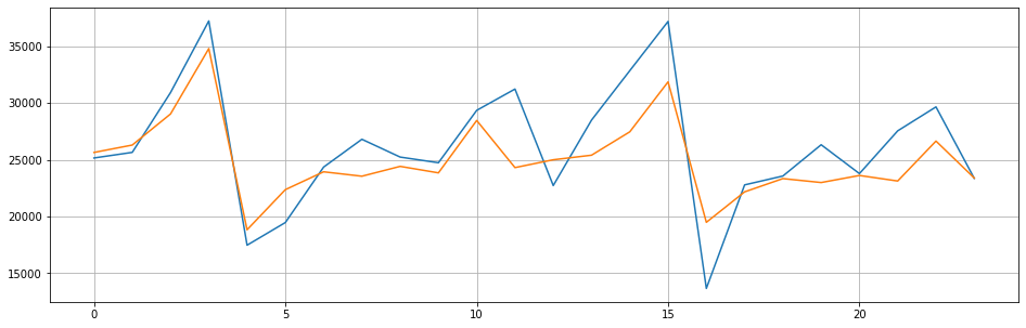
np.sqrt(mean_squared_error(test, model.predict(n_periods=test.shape[0])))3081.3401428137163
model.aic()2936.648256262213
既然pmdarima是基于statsmodel搭建,也能够使用基于R语言的autoarima所有的功能,pmdarima自然也能够支持相应的各类统计学检验以及相关系数计算,更多的详情都可以参考pmdarima的官方说明文档。一般在使用pmdarima建模后,还需要使用统计学中的一系列检验来选择模型、找出能够通过所有检验的模型。
2. 时间序列交叉验证
在时序模型的选择过程中,可以借助交叉验证来帮助我们选择更好的模型。时间序列的交叉验证非常特殊,因为时间序列数据必须遵守“过去预测未来”、“训练中时间顺序不能打乱"等基本原则,因此传统机器学习中的k折交叉验证无法使用。
在时间序列的世界中,有以下两种常见的交叉验证方式:滚动交叉验证(RollingForecastCV) 和滑窗交叉验证 (SlidingWindowForecastCV),当提到“时序交叉验证”时,一般特指滚动交叉验证。下面具体来看一下两种交叉验证的操作:
2.1 滚动交叉验证(RollingForecastCV)
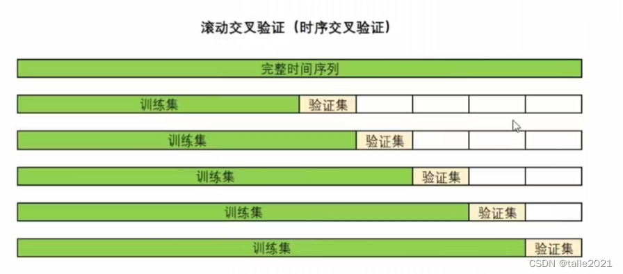
滚动交叉验证是在验证过程中不断增加训练集、并让验证集越来越靠近未来的验证方式,这一方式既能保证我们一定是在用“过去预测未来”,同时也能够保证需要预测的未来和过去真实标签之间的是足够近的,因为越靠近未来的数据对未来的影响越大。这一交叉验证方式很像“多步预测”,但是该方式却不会存在多步预测中的“错误累计"问题,因为在训练过程中我们一直是在使用客观存在的真实标签。
在pmdarima中,我们使用类 RollingForecastCV和 cross_validate 来实现交叉验证,很明显pmdarima的思路借鉴了sklearn (事实上,pmdarima在所有统计学相关内容上是借鉴并依赖于statsmodel进行运行,在所有机器学习相关内容上是借鉴sklearn进行运行)。sklearn中的交叉验证:
cv = KFold(n_splits=5,shuffle=True,random_state=1412)
results = cross_validate(reg,Xtrain,Ytrain,cv=cv)
其中cv是交叉验证具体的模式,cross_validate则负责执行交叉验证本身。在pmdarima运行交叉验证时,类RollingForecastCV的地位等同于普通机器学习交叉验证中的 KFold 类。RollingForecastCv 也只能规定交叉验证的模式,不负责执行交叉验证本身。特别的是,普通K折交叉验证是由折数来控制的,但时序交叉验证其实是以单个样本为单位的。一般来说,时序交叉验证的验证集可以是多个时间点,也可以为单个时间点。当验证集为1个时间点时,滚动交叉验证如下所示:

在pmdarima当中,使用RollingForecastCV来完成交叉验证:
class pmdarima.model selection.RollingForecastCV(h=1,step=1,initial=None)
h:验证集中的样本数量,可以输入[1,n_samples]的整数。
step:训练集中每次增加的样本数量,必须为大于等于1的正整数。
initial:第一次交叉验证时的训练集样本量,如果不填写则按1/3处理。
取h=1,step=1,initial=10
data = pm.datasets.load_wineind()
cv=model_selection.RollingForecastCV(h=1,step=1,initial=10)
cv_generator=cv.split(data)next(cv_generator)#根据initial初始训练集有10个样本,验证集遵循参数h的设置,只包含一个样本(array([0, 1, 2, 3, 4, 5, 6, 7, 8, 9]), array([10]))
next(cv_generator)#根据step的设置,训练集每次增加1个样本,验证集继续包含一个样本(array([ 0, 1, 2, 3, 4, 5, 6, 7, 8, 9, 10]), array([11]))
next(cv_generator)(array([ 0, 1, 2, 3, 4, 5, 6, 7, 8, 9, 10, 11]), array([12]))
取h=10,step=5,initial=10
cv=model_selection.RollingForecastCV(h=10,step=5,initial=10)
cv_generator=cv.split(data)next(cv_generator)(array([0, 1, 2, 3, 4, 5, 6, 7, 8, 9]), array([10, 11, 12, 13, 14, 15, 16, 17, 18, 19]))
next(cv_generator)(array([ 0, 1, 2, 3, 4, 5, 6, 7, 8, 9, 10, 11, 12, 13, 14]), array([15, 16, 17, 18, 19, 20, 21, 22, 23, 24]))
next(cv_generator)(array([ 0, 1, 2, 3, 4, 5, 6, 7, 8, 9, 10, 11, 12, 13, 14, 15, 16,
17, 18, 19]),
array([20, 21, 22, 23, 24, 25, 26, 27, 28, 29]))
不难发现,在pmdarima中实现滚动交叉验证时,验证集实际上是可以重复的,因此滚动交叉验证可以在有限的数据上进行多轮验证集重合的交叉验证,只要满足“过去预测未来”的基本条例,时序交叉验证其实可以相对自由的进行(即验证集与验证集之间不是互斥的)。也因此,时序交叉验证的实际运行时间往往会很长,当数据量巨大时交叉验证的负担也会更大。
# 沿用上面的数据和模型
model=pm.ARIMA(order=(2,1,1),seasonal_order=(1,0,1,12),max_iter=500)
cv=model_selection.RollingForecastCV(h=24,step=12,initial=36)
predictions=model_selection.cross_validate(model,data,cv=cv
                                            ,scoring="mean_squared_error"
                                            ,verbose=2
                                            ,error_score="raise")
[CV] fold=0 .......................................................... [CV] fold=1 .......................................................... [CV] fold=2 .......................................................... [CV] fold=3 .......................................................... [CV] fold=4 .......................................................... [CV] fold=5 .......................................................... [CV] fold=6 .......................................................... [CV] fold=7 .......................................................... [CV] fold=8 .......................................................... [CV] fold=9 ..........................................................
predictions{'test_score': array([1.35362847e+08, 1.08110482e+08, 2.18376249e+07, 1.97805181e+07,
6.16138893e+07, 1.42418110e+07, 1.32432958e+07, 1.31182597e+07,
3.57071218e+07, 5.79654872e+06]),
'fit_time': array([0.2784729 , 0.12543654, 0.62335014, 0.64258695, 0.75659704,
0.73791075, 0.82430649, 0.92007995, 0.98767185, 1.03166628]),
'score_time': array([0.01047397, 0. , 0.00223732, 0. , 0. ,
0. , 0.01564431, 0. , 0.01562428, 0.01562572])}
np.sqrt(predictions["test_score"])array([11634.55400113, 10397.61906654, 4673.07446159, 4447.52944078,
7849.45153132, 3773.83240719, 3639.13393689, 3621.91381986,
5975.54363899, 2407.60227639])
可以看到,交叉验证的测试集中得到的RMSE大部分都大于之前自动化建模时得到的RMSE(2550),并且训练数据越少时,测试集上的RMSE会越大,这可能说明在前几折交叉验证时,训练集的数据量太少,因此可以考虑增大initial当中的设置来避免这个问题。
2.2 滑窗交叉验证(SildingWindowForecastCV)
滑窗交叉验证是借助滑窗技巧完成的交叉验证。滑窗是时间序列中常见的技巧,具体操作如下:
Sliding window——>——>

在时间序列预测时,常常使用窗内的样本作为训练样本、窗右侧(或下方)的第一个样本做为被预测的样本。滑窗技巧在时间序列的各个领域都应用广泛,是时间序列的基础之一。很显然,滑窗交叉验证就是使用窗内的样本作为训练集,窗右侧(或下方)的样本作为验证集而进行的交叉验证。

与滚动交叉验证一样,滑窗交叉验证中的验证集也可以是单一样本,也可以是一系列数据集。相比起滚动交叉验证,滑窗交叉验证的优势在于训练集不会越来越大、每次训练时都使用了理论上对当前验证集来说最有效的信息。但同时,这个优势也会带来问题,由于训练集往往较小,因此滑窗交叉验证需要进行的建模次数异常地多,这可能导致交叉验证模型变得非常缓慢。
在pmdarima当中,使用 SlidingWindowForecastCV 来完成滑窗交叉验证
class pmdarima.model_selection.SlidingWindowForecastCV(h=1,step=1,window size=None)
h:验证集中的样本数量,可以输入[1,n_samples]的整数
step:每次向未来滑窗的样本数量,必须为大于等于1的正整数
window_size:滑窗的尺寸大小,如果填写None则按照样本量整除5得到的数来决定
取h=1,step=1,window_size=10
cv=model_selection.SlidingWindowForecastCV(h=1,step=1,window_size=10)
cv_generator=cv.split(data)
next(cv_generator)#首次进行交叉验证时的数据分割情况
(array([0, 1, 2, 3, 4, 5, 6, 7, 8, 9]), array([10]))
next(cv_generator)#第二次交叉验证时的数据分割情况(array([ 1, 2, 3, 4, 5, 6, 7, 8, 9, 10]), array([11]))
取h=10,step=5,window_size=10
cv=model_selection.SlidingWindowForecastCV(h=10,step=5,window_size=10)
cv_generator=cv.split(data)
next(cv_generator)
(array([0, 1, 2, 3, 4, 5, 6, 7, 8, 9]), array([10, 11, 12, 13, 14, 15, 16, 17, 18, 19]))
next(cv_generator)(array([ 5, 6, 7, 8, 9, 10, 11, 12, 13, 14]), array([15, 16, 17, 18, 19, 20, 21, 22, 23, 24]))
# 沿用上面的数据和模型
model=pm.ARIMA(order=(2,1,1),seasonal_order=(1,0,1,12),max_iter=500)
cv=model_selection.SlidingWindowForecastCV(h=24,step=12,window_size=36)
predictions=model_selection.cross_validate(model,data,cv=cv
                                            ,scoring="mean_squared_error"
                                            ,verbose=2
                                            ,error_score="raise")
[CV] fold=0 .......................................................... [CV] fold=1 .......................................................... [CV] fold=2 .......................................................... [CV] fold=3 .......................................................... [CV] fold=4 .......................................................... [CV] fold=5 .......................................................... [CV] fold=6 .......................................................... [CV] fold=7 .......................................................... [CV] fold=8 .......................................................... [CV] fold=9 ..........................................................
predictions{'test_score': array([1.35362847e+08, 1.20867167e+08, 1.48347243e+08, 2.49879706e+08,
2.32217899e+08, 4.01511152e+08, 1.92061264e+08, 2.51755311e+08,
1.50798724e+08, 1.92747682e+08]),
'fit_time': array([0.28506732, 0.16709971, 0.17653751, 0.12498903, 0.1408143 ,
0.16088152, 0.22708297, 0.33786058, 0.1593399 , 0.27807832]),
'score_time': array([0.00801778, 0. , 0.01562667, 0. , 0.01132369,
0. , 0.01562595, 0. , 0.01562929, 0. ])}
np.sqrt(predictions["test_score"])array([11634.55400113, 10993.96047191, 12179.78831408, 15807.58382521,
15238.69740534, 20037.7431982 , 13858.61697326, 15866.79900091,
12280.01317219, 13883.35991075])
从结果来看,使用更少的训练集进行训练后,模型输出的RMSE大幅上升了,并且也没有变得更稳定,这说明当前模型下更大的训练集会更有利于模型的训练(不是每个时间序列都是这样)。尝试调整滑窗的window_size,就会发现RMSE下降到了与滚动交叉验证时相似的水平:
model=pm.ARIMA(order=(2,1,1),seasonal_order=(1,0,1,12),max_iter=500)
cv=model_selection.SlidingWindowForecastCV(h=24,step=1,window_size=132)
predictions=model_selection.cross_validate(model,data,cv=cv
                                            ,scoring="mean_squared_error"
                                            ,verbose=2
                                            ,error_score="raise")
[CV] fold=0 .......................................................... [CV] fold=1 .......................................................... [CV] fold=2 .......................................................... [CV] fold=3 .......................................................... [CV] fold=4 .......................................................... [CV] fold=5 .......................................................... [CV] fold=6 .......................................................... [CV] fold=7 .......................................................... [CV] fold=8 .......................................................... [CV] fold=9 .......................................................... [CV] fold=10 ......................................................... [CV] fold=11 ......................................................... [CV] fold=12 ......................................................... [CV] fold=13 ......................................................... [CV] fold=14 ......................................................... [CV] fold=15 ......................................................... [CV] fold=16 ......................................................... [CV] fold=17 ......................................................... [CV] fold=18 ......................................................... [CV] fold=19 ......................................................... [CV] fold=20 .........................................................
predictions{'test_score': array([35707121.78143389, 66176325.69903485, 40630659.97659013,
78576782.28645307, 23666490.55159284, 20310751.60353827,
2841898.1720445 , 4484619.0619739 , 18925627.1367884 ,
3231920.46993413, 55955063.23334328, 5769421.1274077 ,
12204785.2577201 , 81763866.37114508, 86166090.62031393,
4308494.01384212, 4472068.45984436, 80544390.23157245,
95444224.35956413, 4356301.4101477 , 41312817.67528097]),
'fit_time': array([0.98685646, 1.00776458, 0.98309445, 0.98523855, 0.99820113,
0.88483882, 1.14556432, 0.94388413, 0.95140123, 1.01311779,
1.01590633, 1.06021142, 1.05152464, 1.06878543, 1.08534598,
1.07379961, 0.96942186, 0.92225981, 0.95834565, 1.33569884,
0.91161823]),
'score_time': array([0.01562262, 0.01562762, 0. , 0.00460625, 0. ,
0.00678897, 0.00810504, 0.01536226, 0.01825047, 0.00629425,
0.00742435, 0.01564217, 0. , 0. , 0. ,
0. , 0.00800204, 0.01618385, 0. , 0.01562595,
0. ])}
np.sqrt(predictions["test_score"])array([5975.54363899, 8134.88326278, 6374.21838162, 8864.35458939,
4864.82173893, 4506.74512298, 1685.79303951, 2117.69191857,
4350.35942616, 1797.75428519, 7480.31170696, 2401.96193296,
3493.53477981, 9042.33743958, 9282.56918209, 2075.69121351,
2114.72656858, 8974.65265242, 9769.55599603, 2087.17546223,
6427.50477832])
此时RMSE的均值大幅下降了,但是模型还是不稳定(波动较大),这说明当前时间序列各时间段上的差异较大,当前模型的拟合结果一般。虽然通过增加训练集的数据量可以让模型表现提升,但极其不稳定的结果展示当前模型的泛化能力是缺失的。和使用AIC时一样,我们只能选择表现更好的时序模型(只能择优),而无法选择完美的时序模型。当我们将auto_arima选出的最佳参数放弃、而选择带有其他参数的模型,说不定得到的结果会更加不稳定。
你是否注意到一个细节?时序交叉验证不会返回训练集上的分数,同时pmdarima的预测功能predict中也不接受对过去进行预测。通常来说我们判断过拟合的标准是训练集上的结果远远好于测试集,但时序交叉验证却不返回训练集分数,因此时间序列数据无法通过对比训练集和测试集结果来判断是否过拟合。但在时间序列的世界中,依然存在着”过拟合”这个概念,我们可以通过交叉验证的结果来判断不同参数下的时间序列模型哪个过拟合程度更轻。
通常来说,验证集上的分数最佳的模型过拟合风险往往最小,因为当一个模型学习能够足够强、且既不过拟合又不欠拟合的时候,模型的训练集和验证集分数应该是高度接近的,所以验证集分数越好,验证集的分数就越可能更接近训练集上的分数。因此在多个模型对比的情况下,我们可以只通过观察测试集上的分数来选定最佳模型。这个最佳模型即是表现最佳的模型,也是过拟合风险最小的模型(不是绝对)。