目录
以面板数据mus08psidextract.dta为例:
1.导入数据集
stata自带数据集:Stata打开自带的数据合集_9997PZ的博客-CSDN博客_stata数据
外部导入:
. use "F:\个人嘿嘿嘿\北师大BNU\研一上-课业资料\商务与经济统计\作业1\mus08psidextract.dta",clear 2.面板数据有关信息
面板数据是一种多维数据,一般具有两个维度:个体(组、类)和时间。
面板数据既含有n个个体截面的数据,也含有长为T的时间序列。
2.1设定面板数据的个体变量和时间变量
. xtset id t   //id:个体变量 t:时间变量 顺序不可以变
Panel variable: id (strongly balanced)
 Time variable: t, 1 to 7
         Delta: 1 unit
2.2显示面板数据的结构:
. xtdes
2.3显示数据集中变量的统计特征:
. xtsum
. xtsum lwage ed exp exp2 wks id t

Variable         |      Mean   Std. dev.       Min        Max |    Observations
-----------------+--------------------------------------------+----------------
lwage    overall |  6.676346   .4615122    4.60517      8.537 |     N =    4165
         between |             .3942387     5.3364   7.813596 |     n =     595
         within  |             .2404023   4.781808   8.621092 |     T =       7
                 |                                            |
ed       overall |  12.84538   2.787995          4         17 |     N =    4165
         between |             2.790006          4         17 |     n =     595
         within  |                    0   12.84538   12.84538 |     T =       7
                 |                                            |
exp      overall |  19.85378   10.96637          1         51 |     N =    4165
         between |             10.79018          4         48 |     n =     595
         within  |              2.00024   16.85378   22.85378 |     T =       7
                 |                                            |
exp2     overall |   514.405   496.9962          1       2601 |     N =    4165
         between |             489.0495         20       2308 |     n =     595
         within  |             90.44581    231.405    807.405 |     T =       7
                 |                                            |
wks      overall |  46.81152   5.129098          5         52 |     N =    4165
         between |             3.284016   31.57143   51.57143 |     n =     595
         within  |             3.941881    12.2401   63.66867 |     T =       7
                 |                                            |
id       overall |       298   171.7821          1        595 |     N =    4165
         between |              171.906          1        595 |     n =     595
         within  |                    0        298        298 |     T =       7
                 |                                            |
t        overall |         4    2.00024          1          7 |     N =    4165
         between |                    0          4          4 |     n =     595
         within  |              2.00024          1          7 |     T =       7

.
std.dev:基于样本估算标准偏差,反映数值相对于平均值的离散程度;
可以看出id的组内离散程度为0(同一个体内,个体无变化),t的组间离散程度为0(同一时间,每一个个体之间时间无差别);ed可以看作,是可以观测到的个体异质性;
3.混合回归
. reg y x1 x2 x3…,vce(cluster id)
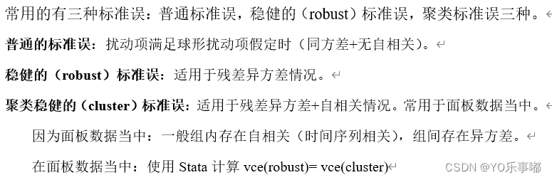
其中vce(cluster id)【聚类标准误】可替换为:robust / r【稳健标准误】 or 什么都不加【普通标准误】,下面各种模型回归同理。
注:_cons为默认加入的常数项,如果要求不含常数项则使用:reg y x1 x2 x3…,nocons
reg lwage exp exp2 wks ed,vce(cluster id)  //使用聚类稳健标准误

Linear regression                               Number of obs     =      4,165
                                                F(4, 594)         =      72.58
                                                Prob > F          =     0.0000
                                                R-squared         =     0.2836
                                                Root MSE          =     .39082

                                   (Std. err. adjusted for 595 clusters in id)
------------------------------------------------------------------------------
             |               Robust
       lwage | Coefficient  std. err.      t    P>|t|     [95% conf. interval]
-------------+----------------------------------------------------------------
         exp |    .044675   .0054385     8.21   0.000     .0339941     .055356
        exp2 |  -.0007156   .0001285    -5.57   0.000    -.0009679   -.0004633
         wks |    .005827   .0019284     3.02   0.003     .0020396    .0096144
          ed |   .0760407   .0052122    14.59   0.000     .0658042    .0862772
       _cons |   4.907961   .1399887    35.06   0.000     4.633028    5.182894
------------------------------------------------------------------------------
4.随机效应模型
4.1随机效应模型or混合回归模型的选择:LM检验
LM检验 检验是否存在个体效应 从而确定使用
(使用FGLS法会提供一个theta值,从而完成LM检验)
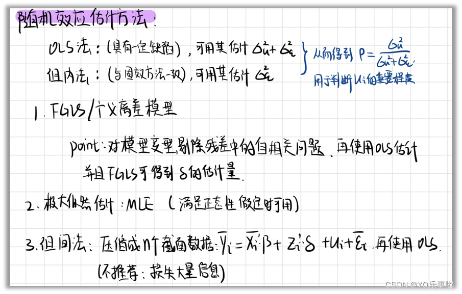
4.2随机效应模型:两种估计方法
A.FGLS法:广义离差模型
. xtreg y x1 x2…, re r theta
. xtreg lwage exp exp2 wks ed, re r theta

Random-effects GLS regression                   Number of obs     =      4,165
Group variable: id                              Number of groups  =        595

R-squared:                                      Obs per group:
     Within  = 0.6340                                         min =          7
     Between = 0.1716                                         avg =        7.0
     Overall = 0.1830                                         max =          7

                                                Wald chi2(4)      =    1598.50
corr(u_i, X) = 0 (assumed)                      Prob > chi2       =     0.0000
theta        = .82280511

                                   (Std. err. adjusted for 595 clusters in id)
------------------------------------------------------------------------------
             |               Robust
       lwage | Coefficient  std. err.      z    P>|z|     [95% conf. interval]
-------------+----------------------------------------------------------------
         exp |   .0888609   .0039992    22.22   0.000     .0810227    .0966992
        exp2 |  -.0007726   .0000896    -8.62   0.000    -.0009481    -.000597
         wks |   .0009658   .0009259     1.04   0.297     -.000849    .0027806
          ed |   .1117099   .0083954    13.31   0.000     .0952552    .1281647
       _cons |   3.829366   .1333931    28.71   0.000     3.567921    4.090812
-------------+----------------------------------------------------------------
     sigma_u |  .31951859
     sigma_e |  .15220316
         rho |  .81505521   (fraction of variance due to u_i)
------------------------------------------------------------------------------
可以看到theta=0.8228,LM检验中:强烈拒绝“不存在个体随机效应”的原假设,个体效应存在,在混合回归和随机效应模型当中应该选择随机效应模型;
rho=0.8151 进一步证明ui部分在方程中起到重要的作用,是不可以被忽略的;
B.MLE法:极大似然估计
当扰动项服从正态分布时,可以使用此方法。
. xtreg y x1 x2 x3…,mle
4.3双向随机效应模型
FGLS(估计个体效应)+LSDV法(估计时间效应)估计
. xtreg y x1 x2 x3…i.year,re
5.固定效应模型
5.1固定效应模型or混合回归之间的选择:
H0:all ui=0
普通标准误的估计时会给出一个F检验结果:F=53.12 p=0.000 则拒绝原假设,即应当使用固定效应模型
5.2固定效应模型估计方法
A.组内法:FE
. xtreg y x1 x2…, fe
缺点:无法估计出可观测的个体异质性的系数
,所以下表中ed 为omitted状态
注意:xtreg下r(robust)等价于聚类稳健标准误
. xtreg lwage exp exp2 wks ed, fe //普通标准误
note: ed omitted because of collinearity.

Fixed-effects (within) regression               Number of obs     =      4,165
Group variable: id                              Number of groups  =        595

R-squared:                                      Obs per group:
     Within  = 0.6566                                         min =          7
     Between = 0.0276                                         avg =        7.0
     Overall = 0.0476                                         max =          7

                                                F(3,3567)         =    2273.74
corr(u_i, Xb) = -0.9107                         Prob > F          =     0.0000

------------------------------------------------------------------------------
       lwage | Coefficient  Std. err.      t    P>|t|     [95% conf. interval]
-------------+----------------------------------------------------------------
         exp |   .1137879   .0024689    46.09   0.000     .1089473    .1186284
        exp2 |  -.0004244   .0000546    -7.77   0.000    -.0005315   -.0003173
         wks |   .0008359   .0005997     1.39   0.163    -.0003399    .0020116
          ed |          0  (omitted)
       _cons |   4.596396   .0389061   118.14   0.000     4.520116    4.672677
-------------+----------------------------------------------------------------
     sigma_u |  1.0362039
     sigma_e |  .15220316
         rho |  .97888036   (fraction of variance due to u_i)
------------------------------------------------------------------------------
F test that all u_i=0: F(594, 3567) = 53.12                  Prob > F = 0.0000
. xtreg lwage exp exp2 wks ed, fe vce(cluster id) //聚类稳健标准误
note: ed omitted because of collinearity.

Fixed-effects (within) regression               Number of obs     =      4,165
Group variable: id                              Number of groups  =        595

R-squared:                                      Obs per group:
     Within  = 0.6566                                         min =          7
     Between = 0.0276                                         avg =        7.0
     Overall = 0.0476                                         max =          7

                                                F(3,594)          =    1059.72
corr(u_i, Xb) = -0.9107                         Prob > F          =     0.0000

                                   (Std. err. adjusted for 595 clusters in id)
------------------------------------------------------------------------------
             |               Robust
       lwage | Coefficient  std. err.      t    P>|t|     [95% conf. interval]
-------------+----------------------------------------------------------------
         exp |   .1137879   .0040289    28.24   0.000     .1058753    .1217004
        exp2 |  -.0004244   .0000822    -5.16   0.000    -.0005858   -.0002629
         wks |   .0008359   .0008697     0.96   0.337    -.0008721    .0025439
          ed |          0  (omitted)
       _cons |   4.596396   .0600887    76.49   0.000     4.478384    4.714408
-------------+----------------------------------------------------------------
     sigma_u |  1.0362039
     sigma_e |  .15220316
         rho |  .97888036   (fraction of variance due to u_i)
------------------------------------------------------------------------------
B.LSDV法
. reg y x1 x2 x3…i.id,vce(cluster id)
i.id:表示根据变量id而产生的虚拟变量,生成n个虚拟变量(or 有截距项时生成n-1个)
优点:可以求出可观测的个体异质性的系数
C.一阶差分法FD
无专门命令,可以使用一些其他方法来附带进行(?待补充)
5.3.双向固定效应模型LSDV法
法一:. xtreg y x1 x2…i.year, fe r
法二:. reg lwage exp exp2 wks ed i.id i.year, robust
若数据未变形:(如把1976-1982转为1-7)
. tab year,gen(year)
若数据已经为标准形式,则直接使用
. xtreg lwage exp exp2 wks ed i.t, fe r
note: ed omitted because of collinearity.
note: 7.t omitted because of collinearity.

Fixed-effects (within) regression               Number of obs     =      4,165
Group variable: id                              Number of groups  =        595

R-squared:                                      Obs per group:
     Within  = 0.6599                                         min =          7
     Between = 0.0275                                         avg =        7.0
     Overall = 0.0480                                         max =          7

                                                F(8,594)          =     412.33
corr(u_i, Xb) = -0.9089                         Prob > F          =     0.0000

                                   (Std. err. adjusted for 595 clusters in id)
------------------------------------------------------------------------------
             |               Robust
       lwage | Coefficient  std. err.      t    P>|t|     [95% conf. interval]
-------------+----------------------------------------------------------------
         exp |   .1119927   .0041184    27.19   0.000     .1039043    .1200812
        exp2 |  -.0004051   .0000834    -4.86   0.000    -.0005688   -.0002413
         wks |     .00068   .0008812     0.77   0.441    -.0010506    .0024105
          ed |          0  (omitted)
             |
           t |
          2  |  -.0083984   .0049321    -1.70   0.089    -.0180849    .0012881
          3  |   .0259652   .0084359     3.08   0.002     .0093974    .0425329
          4  |   .0289134   .0078093     3.70   0.000     .0135762    .0442506
          5  |   .0239406   .0065275     3.67   0.000     .0111208    .0367604
          6  |   .0069955   .0064617     1.08   0.279    -.0056949     .019686
          7  |          0  (omitted)
             |
       _cons |   4.618339   .0599451    77.04   0.000     4.500609    4.736069
-------------+----------------------------------------------------------------
     sigma_u |  1.0268811
     sigma_e |  .15159041
         rho |  .97867247   (fraction of variance due to u_i)
------------------------------------------------------------------------------
6.豪斯曼检验:固定效应模型or随机效应模型
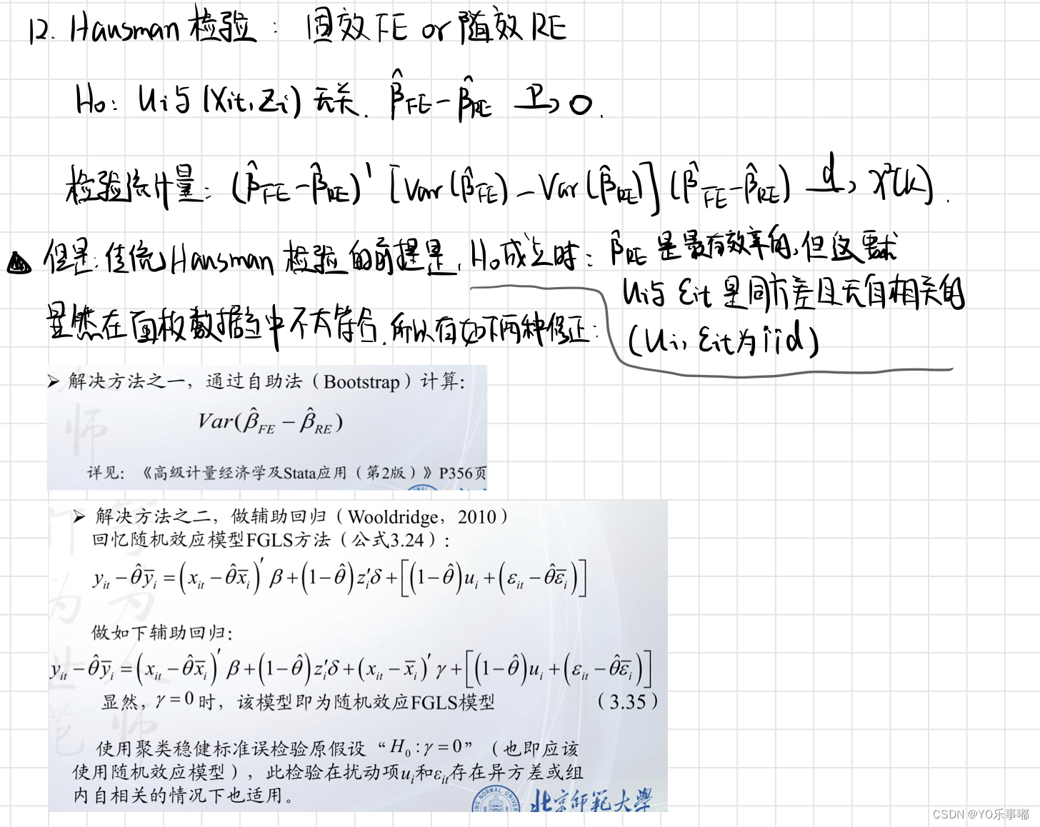
6.1传统Hausman检验
(前提:ui与eit是独立同分布的)
. xtreg lwage exp exp2 wks ed, fe
. estimates store FE
. xtreg lwage exp exp2 wks ed, re theta
. estimates store RE
. hausman FE RE,constant sigmamore
注:必须使用普通标准误,不可以使用稳健标准误
若原假设成立,则认为ui与xi和eit无相关性,应当使用随机效应模型;
. hausman FE RE,constant sigmamore

                 ---- Coefficients ----
             |      (b)          (B)            (b-B)     sqrt(diag(V_b-V_B))
             |       FE           RE         Difference       Std. err.
-------------+----------------------------------------------------------------
         exp |    .1137879     .0888609        .0249269        .0012778
        exp2 |   -.0004244    -.0007726        .0003482        .0000285
         wks |    .0008359     .0009658       -.0001299        .0001108
       _cons |    4.596396     3.829366        .7670299               .
------------------------------------------------------------------------------
                          b = Consistent under H0 and Ha; obtained from xtreg.
           B = Inconsistent under Ha, efficient under H0; obtained from xtreg.

Test of H0: Difference in coefficients not systematic

    chi2(4) = (b-B)'[(V_b-V_B)^(-1)](b-B)
            = 1374.55
Prob > chi2 =  0.0000
(V_b-V_B is not positive definite)

.
由结果来看p值为0.0000则强烈拒绝原假设,应当选择固定个体效应模型;
再对时间效应进行检验(?应当比较时间固定模型还是直接比较双向固定模型
6.2非传统Hausman检验
前提:ui与eit都不再是iid情况下
即当聚类稳健标准误与普通标准误相差较大时,显然不再满去传统Hausman检验的前提,此时要使用另一种方法:
H0:=0
. ssc install xtoverid
. xtreg y x1 x2 …,re r //先运行聚类稳健标准误的RE
. xtoverid
. xtoverid //非传统豪斯曼检验

Test of overidentifying restrictions: fixed vs random effects
Cross-section time-series model: xtreg re  robust cluster(id)
Sargan-Hansen statistic 1792.412  Chi-sq(3)   P-value = 0.0000
-----22.12.8 在期末复习(苦涩)补充一些知识点-----
7.理论知识点补充
7.1一般建模流程(待完善补充)

7.2三种标准误
7.3FE与RE的估计方法总结
7.3.1固定效应模型:组内法、LSDV法、差分法

7.3.2随机效应模型估计方法:广义离差模型FGLS法、极大似然估计
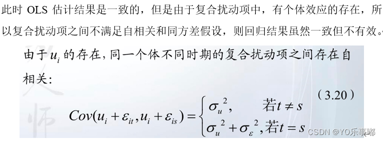
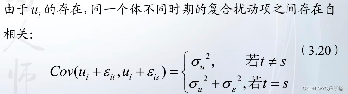
此时OLS估计结果是一致的,但是由于复合扰动项中,有个体效应的存在,所以复合扰动项之间不满足自相关和同方差假设,则OLS回归结果虽然一致但不有效。
7.4工具变量辅助检验
面板数据的内生性问题:
虽然面板数据的个体异质性可以一定程度上缓解遗漏变量问题,但是模型仍然可能存在内生性(测量误差、模型误设、双向因果等)。此时可以使用工具变量法。
7.4.1(固定效应模型)使用IV的步骤:
Step1:对模型变换以缓解遗漏变量的影响,模型组内离差(或一阶差分);
Step2:再使用IV,做2SLS;
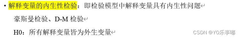
7.4.2工具变量四个辅助检验

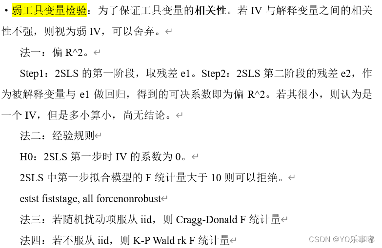
7.5动态面板数据
动态面板数据PDP:指解释变量中包含被解释变量的滞后项。
是解决内生性问题的最后手段:用于解决遗漏变量以及双向因果导致的内生性。
三种常用估计方法:差分GMM、水平GMM、系统GMM。