Stata将回归分析结果直接导出到Word里
ssc install asdoc, replace
写每个命令时前面加上asdoc就可将生成的结果存在word 中
将图片保存成.emf格式,可在word中直接插入。
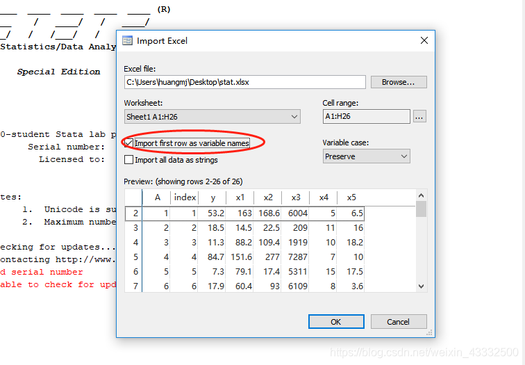
导入数据
数据描述
. sum#描述数据

    Variable |        Obs        Mean    Std. Dev.       Min        Max
-------------+---------------------------------------------------------
           A |         25          13    7.359801          1         25
       index |         25          13    7.359801          1         25
           y |         25      26.444    24.60308        1.9       84.7
          x1 |         25     101.032    64.96047       13.2      299.5
          x2 |         25      99.384    63.28338        6.1        277
-------------+---------------------------------------------------------
          x3 |         25      5197.4    3649.682        209      15571
          x4 |         25        11.4    7.112196          2         34
          x5 |         25      11.848    7.625676        2.5       33.7
由上表可以看出每个变量的最大值,最小值,平均值,标准差以及样本个数等具体值。
describe#描述数据,和sum有一定区别
得到
Contains data
  obs:            25
 vars:             8
 size:           925
-----------------------------------------------------------------------------------------------
              storage   display    value
variable name   type    format     label      variable label
-----------------------------------------------------------------------------------------------
A               byte    %10.0g
index           byte    %10.0g                index
y               double  %10.0g                y
x1              double  %10.0g                x1
x2              double  %10.0g                x2
x3              int     %10.0g                x3
x4              byte    %10.0g                x4
x5              double  %10.0g                x5
-----------------------------------------------------------------------------------------------
Sorted by:
     Note: Dataset has changed since last saved.
得到样本数据特征
线性回归
regress y x1 x2 x3 x4 x5#作线性回归
结果
      Source |       SS           df       MS      Number of obs   =        25
-------------+----------------------------------   F(5, 19)        =     21.84
       Model |  12374.4556         5  2474.89112   Prob > F        =    0.0000
    Residual |  2153.02602        19  113.317159   R-squared       =    0.8518
-------------+----------------------------------   Adj R-squared   =    0.8128
       Total |  14527.4816        24  605.311733   Root MSE        =    10.645

------------------------------------------------------------------------------
           y |      Coef.   Std. Err.      t    P>|t|     [95% Conf. Interval]
-------------+----------------------------------------------------------------
          x1 |   .1273254    .095979     1.33   0.200     -.073561    .3282118
          x2 |    .160566   .0556834     2.88   0.010     .0440194    .2771126
          x3 |   .0007636   .0013556     0.56   0.580    -.0020737    .0036009
          x4 |   -.333199   .3986248    -0.84   0.414     -1.16753    .5011323
          x5 |  -.5746462   .3087506    -1.86   0.078    -1.220869    .0715763
       _cons |   4.260477   10.46798     0.41   0.689    -17.64926    26.17022
------------------------------------------------------------------------------
相关系数矩阵
correlate y x1 x2 x3 x4 x5
             |        y       x1       x2       x3       x4       x5
-------------+------------------------------------------------------
           y |   1.0000
          x1 |   0.8505   1.0000
          x2 |   0.8332   0.7381   1.0000
          x3 |   0.7409   0.8832   0.5534   1.0000
          x4 |  -0.6043  -0.6231  -0.5382  -0.5225   1.0000
          x5 |  -0.4470  -0.2775  -0.3231  -0.2910   0.0953   1.0000
##Stata检查是否存在多重共线性
用容忍度和方差膨胀因子(VIF),VIF 大于10 存在严重的共线性,若自变量间存在的多重相关性这里将采取逐步回归法进行修正。
estat vif
    Variable |       VIF       1/VIF
-------------+----------------------
          x1 |      8.23    0.121460
          x3 |      5.18    0.192888
          x2 |      2.63    0.380237
          x4 |      1.70    0.587420
          x5 |      1.17    0.851750
-------------+----------------------
    Mean VIF |      3.78
pca x1 x2 x3 x4 x5
Principal components/correlation                 Number of obs    =         25
                                                 Number of comp.  =          5
                                                 Trace            =          5
    Rotation: (unrotated = principal)            Rho              =     1.0000

    --------------------------------------------------------------------------
       Component |   Eigenvalue   Difference         Proportion   Cumulative
    -------------+------------------------------------------------------------
           Comp1 |      3.06752      2.13626             0.6135       0.6135
           Comp2 |      .931263       .42405             0.1863       0.7998
           Comp3 |      .507212     .0891979             0.1014       0.9012
           Comp4 |      .418014      .342028             0.0836       0.9848
           Comp5 |     .0759864            .             0.0152       1.0000
    --------------------------------------------------------------------------

Principal components (eigenvectors)

    ------------------------------------------------------------------------------
        Variable |    Comp1     Comp2     Comp3     Comp4     Comp5 | Unexplained
    -------------+--------------------------------------------------+-------------
              x1 |   0.5411    0.0950    0.2986    0.0764   -0.7767 |           0
              x2 |   0.4736   -0.0361   -0.3527    0.7615    0.2648 |           0
              x3 |   0.4981    0.0407    0.6165   -0.2196    0.5674 |           0
              x4 |  -0.4231   -0.3830    0.6107    0.5463   -0.0531 |           0
              x5 |  -0.2362    0.9172    0.1828    0.2600    0.0435 |           0
    ------------------------------------------------------------------------------