1. 画图函数
%matplotlib inline
import matplotlib.pyplot as plt
def runplt():
    plt.figure()
    plt.title('diameter-cost curver')
    plt.xlabel('diameter')
    plt.ylabel('cost')
    plt.axis([0, 25, 0, 25])
    plt.grid(True)
    return plt

plt = runplt()
X = [[6], [8], [10], [14], [18]]
y = [[7], [9], [13], [17.5], [18]]
plt.plot(X, y, 'k.')
plt.show()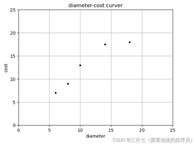
2. 预测价格
from sklearn.linear_model import LinearRegression
import numpy as np
# 创建并拟合模型
model = LinearRegression()
model.fit(X, y)
print('预测12英寸匹萨价格:$%.2f' % model.predict(np.array([12]).reshape(-1, 1))[0])
model = LinearRegression() :初始化一个线性回归模型的实例。
然后可以使用这个模型来:
训练模型:使用 .fit() 方法,传入特征数据 X 和标签数据 y
预测:使用 .predict() 方法,传入新的特征数据,得到预测结果
查看模型参数(权重):通过 .coef_ 和 .intercept_ 属性
fit() 方法用于使用给定的输入特征 X 和相应的目标值 y 对模型进行训练。输入特征 X 应该
是一个二维数组对象,比如一个 NumPy 或者一个 DataFrame,其中每一行表示一个样本,每一列
表示一个特征。目标值 y 应该是一个一维数组对象,比如一个 NumPy 或者一个 Pandas Series,
包含每个样本对应的目标值。
reshape(-1, 1) 的目的是将一个一维数组或向量转换为一个列向量。参数 -1 表示根据数组
的大小自动计算维度,而 1 表示结果数组应该是一个列向量。np.array([12]).reshape(-1, 1) 创
建了一个包含单个值12的NumPy数组,并将其重塑为一个列向量。然后,通过调用 predict() 方
法并传入这个重塑后的输入特征,对其进行预测。predict() 方法返回预测结果,通过索引 [0] 取
得了预测结果的第一个元素。所以整段代码的目的是使用模型对输入特征值12进行预测,并返回预
测结果的第一个元素。
plt = runplt()
plt.plot(X, y, 'k.')
X2 = [[0], [10], [14], [25]]
model = LinearRegression()
model.fit(X, y)
y2 = model.predict(X2)
plt.plot(X, y, 'k.')
plt.plot(X2, y2, 'g-')
plt.show()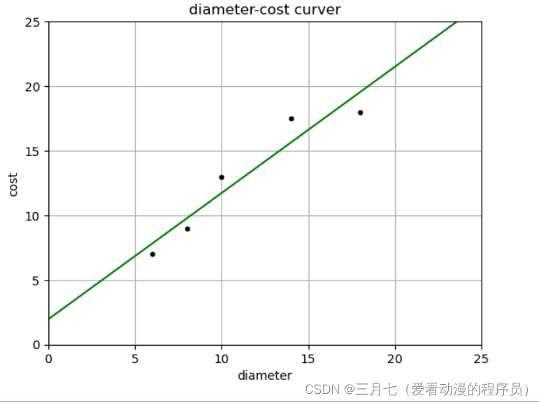
plt = runplt()
plt.plot(X, y, 'k.')
X2 = [[0], [10], [14], [25]]
model = LinearRegression()
model.fit(X, y)
y2 = model.predict(X2)

plt.plot(X2, y2, 'g-')

# 残差预测值
yr = model.predict(X)
for idx, x in enumerate(X):
    plt.plot([x, x], [y[idx], yr[idx]], 'r-')

plt.show()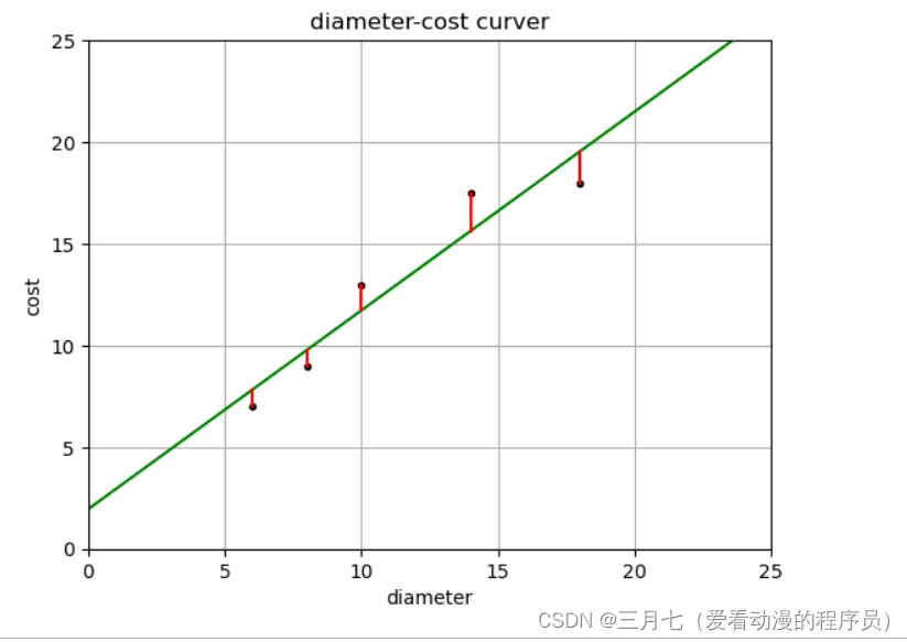
print('残差平方和: %.2f' % np.mean((model.predict(X) - y) ** 2))
# 残差平方和: 1.75
3. 线性回归
from sklearn.linear_model import LinearRegression
X = [[6, 2], [8, 1], [10, 0], [14, 2], [18, 0]]
y = [[7], [9], [13], [17.5], [18]]
model = LinearRegression()
model.fit(X, y)
X_test = [[8, 2], [9, 0], [11, 2], [16, 2], [12, 0]]
y_test = [[11], [8.5], [15], [18], [11]]
predictions = model.predict(X_test)
for i, prediction in enumerate(predictions):
    print('Predicted: %s, Target: %s' % (prediction, y_test[i]))
print('R-squared: %.2f' % model.score(X_test, y_test))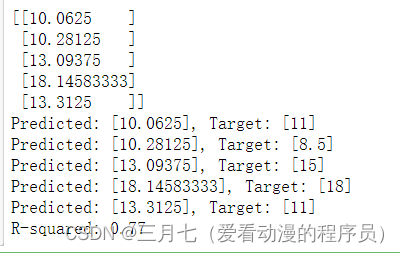
enumerate() 是一个内置函数,用于在迭代过程中同时获取元素的索引和值。
当你使用 enumerate(iterable) 时,它会返回一个迭代器对象,该对象生成元组 (index,
value),其中 index 是元素在迭代过程中的索引,value 是对应的元素值。
使用 enumerate() 可以方便地在循环中同时获取索引和值,特别适用于需要追踪元素位置的情况,
例如在处理列表、字符串等可迭代对象时。
import numpy as np
from sklearn.linear_model import LinearRegression
from sklearn.preprocessing import PolynomialFeatures
X_train = [[6], [8], [10], [14], [18]]
y_train = [[7], [9], [13], [17.5], [18]]
X_test = [[6], [8], [11], [16]]
y_test = [[8], [12], [15], [18]]
# 建立线性回归,并用训练的模型绘图
regressor = LinearRegression()
regressor.fit(X_train, y_train)
xx = np.linspace(0, 26, 100)
yy = regressor.predict(xx.reshape(xx.shape[0], 1))
plt = runplt()
plt.plot(X_train, y_train, 'k.')
plt.plot(xx, yy)
quadratic_featurizer = PolynomialFeatures(degree=2)
X_train_quadratic = quadratic_featurizer.fit_transform(X_train)
X_test_quadratic = quadratic_featurizer.transform(X_test)
regressor_quadratic = LinearRegression()
regressor_quadratic.fit(X_train_quadratic, y_train)
xx_quadratic = quadratic_featurizer.transform(xx.reshape(xx.shape[0], 1))
plt.plot(xx, regressor_quadratic.predict(xx_quadratic), 'r-')
plt.show()
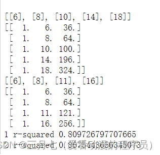
print(X_train)
print(X_train_quadratic)
print(X_test)
print(X_test_quadratic)
print('1 r-squared', regressor.score(X_test, y_test))
print('2 r-squared', regressor_quadratic.score(X_test_quadratic, y_test)) 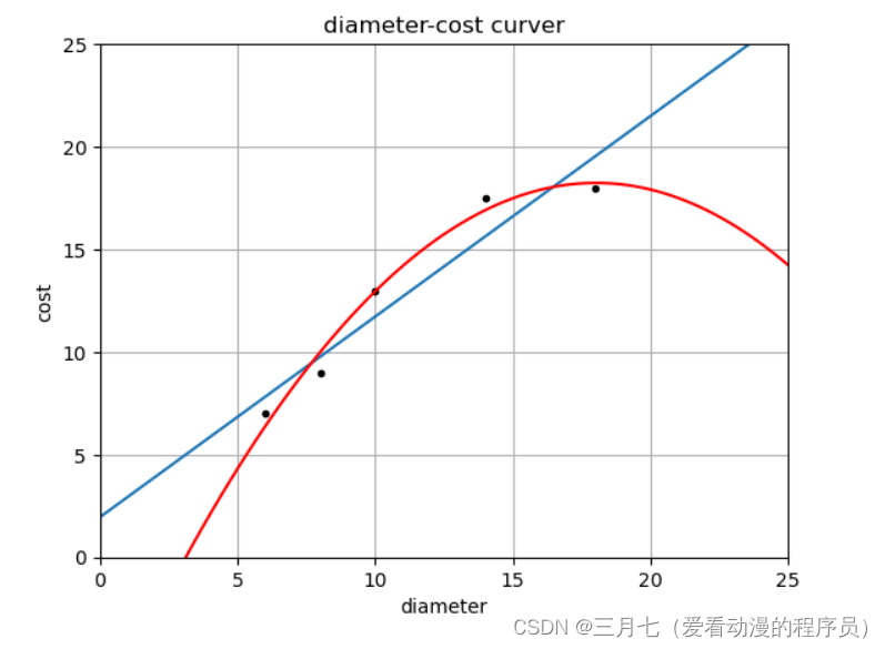
linspace(0, 26, 100) 生成了一个包含 100 个数字的数组,这些数字从 0 开始,到 26 结
束,且在这个范围内均匀地分布。
reshape(xx.shape[0], 1) 的目的是将数组 xx 重塑为一个列向量。xx 是一个一维数组,通
过调用 reshape() 方法,并传入参数 (xx.shape[0], 1),将其转换为一个二维数组,其中
有 xx.shape[0] 行,1 列。xx.shape[0] 表示数组 xx 的长度,即元素的个数。通过将数组重塑
为 (xx.shape[0], 1) 的形状,我们将其转换为一个列向量,其中每个元素都在单独的行中。
quadratic_featurizer = PolynomialFeatures(degree=2) 是用于生成二次多项式特征的
PolynomialFeatures 类的实例化操作。PolynomialFeatures 是 Scikit-learn 库中的一个函数,用于
生成多项式特征。通过指定 degree 参数,可以控制生成多项式的最高次数。在这个例子中,通过
将 degree 参数设置为 2,创建了一个二次多项式特征生成器的实例 quadratic_featurizer。生成的
二次多项式特征可以用于回归或分类模型的训练。例如,可以将这些特征输入到线性回归模型
中,以拟合一个二次曲线。接下来,可以使用 quadratic_featurizer 对数据进行转换,将原始特
征转换为二次多项式特征。使用 fit_transform() 方法可以同时进行拟合和转换,生成新的特征矩
阵。
在使用 PolynomialFeatures 类对训练集和测试集的特征进行二次多项式特征转换时,首先,
通过调用 quadratic_featurizer.fit_transform(X_train),对训练集的特征 X_train 进行拟合和
转换,生成一个包含原始特征及其二次交互项的新特征矩阵 X_train_quadratic。这个新特征矩阵将
用于训练模型。
然后,通过调用 quadratic_featurizer.transform(X_test),对测试集的特征 X_test 进行
转换,生成一个与训练集特征矩阵具有相同形状的新特征矩阵 X_test_quadratic。这个新特征矩阵
将用于在训练好的模型上进行预测或评估。
使用 fit_transform() 方法在训练集上进行拟合和转换的目的是确保生成的新特征矩阵包含
训练集中所有可能的特征组合。然后,使用 transform() 方法在测试集上进行转换,以保持特征的
一致性。这样做的目的是在训练和测试阶段使用相同的特征转换方式,确保模型在处理新数据时具
有相同的特征表示。这有助于避免模型在训练和测试数据之间出现不一致的特征表示问题。
通过调用 score(X_test, y_test) 方法,可以计算回归模型在测试集上的拟合度量得分。这
个得分通常用来评估模型的性能和预测的准确性。具体得分的计算方式取决于所使用的回归模型。
对于大多数回归模型,这个得分是 R-squared(决定系数)的值,其范围从 0 到 1,表示模型对目
标变量的解释能力。R-squared 的值越接近 1,表示模型对目标变量的解释能力越强,拟合效果越
好。而值越接近 0,表示模型对目标变量的解释能力较弱,拟合效果较差。R-squared 是一种常见
的拟合度量分数。它表示模型对目标变量的解释能力。R-squared 的计算方式是通过比较模型预测
的方差和目标变量的方差来衡量。
plt = runplt()
plt.plot(X_train, y_train, 'k.')
quadratic_featurizer = PolynomialFeatures(degree=2)
X_train_quadratic = quadratic_featurizer.fit_transform(X_train)
X_test_quadratic = quadratic_featurizer.transform(X_test)
regressor_quadratic = LinearRegression()
regressor_quadratic.fit(X_train_quadratic, y_train)
xx_quadratic = quadratic_featurizer.transform(xx.reshape(xx.shape[0], 1))
plt.plot(xx, regressor_quadratic.predict(xx_quadratic), 'r-')
cubic_featurizer = PolynomialFeatures(degree=3)
X_train_cubic = cubic_featurizer.fit_transform(X_train)
X_test_cubic = cubic_featurizer.transform(X_test)
regressor_cubic = LinearRegression()
regressor_cubic.fit(X_train_cubic, y_train)
xx_cubic = cubic_featurizer.transform(xx.reshape(xx.shape[0], 1))
plt.plot(xx, regressor_cubic.predict(xx_cubic))
plt.show()
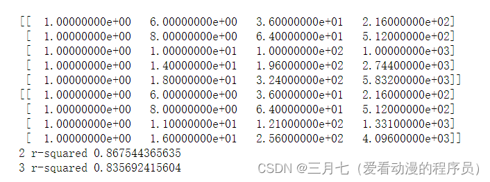
print(X_train_cubic)
print(X_test_cubic)
print('2 r-squared', regressor_quadratic.score(X_test_quadratic, y_test))
print('3 r-squared', regressor_cubic.score(X_test_cubic, y_test))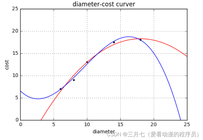
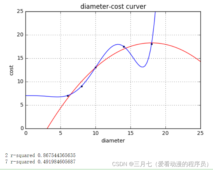
plt = runplt()
plt.plot(X_train, y_train, 'k.')

quadratic_featurizer = PolynomialFeatures(degree=2)
X_train_quadratic = quadratic_featurizer.fit_transform(X_train)
X_test_quadratic = quadratic_featurizer.transform(X_test)
regressor_quadratic = LinearRegression()
regressor_quadratic.fit(X_train_quadratic, y_train)
xx_quadratic = quadratic_featurizer.transform(xx.reshape(xx.shape[0], 1))
plt.plot(xx, regressor_quadratic.predict(xx_quadratic), 'r-')

seventh_featurizer = PolynomialFeatures(degree=7)
X_train_seventh = seventh_featurizer.fit_transform(X_train)
X_test_seventh = seventh_featurizer.transform(X_test)
regressor_seventh = LinearRegression()
regressor_seventh.fit(X_train_seventh, y_train)
xx_seventh = seventh_featurizer.transform(xx.reshape(xx.shape[0], 1))
plt.plot(xx, regressor_seventh.predict(xx_seventh))
plt.show()
print('2 r-squared', regressor_quadratic.score(X_test_quadratic, y_test))
print('7 r-squared', regressor_seventh.score(X_test_seventh, y_test))