目录
cost function :代价函数或者损失函数——衡量模型优劣的一个指标
梯度下降——自动寻找最小的cost function 代价函数
实现一个简单的监督学习的模型:预测part1 中提到的买房模型。
模型中有一个输入参数:房子面积 (单位:1000平方)x;一个输出结果:房子价格:y(单位:千美元)
目前假设训练数据有两个:
- 1000平方米的房子,售价300万美元
- 2000平方米的房子,售价500万美元
x_train = np.array([1.0, 2.0])   #features
y_train = np.array([300.0, 500.0])   #target value
训练数据的图像是:
# 绘制训练数据
# Plot the data points
plt.scatter(x_train, y_train, marker='x', c='r')
# Set the title
plt.title("Housing Prices")
# Set the y-axis label
plt.ylabel('Price (in 1000s of dollars)')
# Set the x-axis label
plt.xlabel('Size (1000 sqft)')
plt.show()

x_train中保存的是房子面积的集合,y_train中保存的是对应面积房子的价格
线性模型实现:
首先,线性模型的计算公式是y = w*x+b,其中x是输入变量,y输出变量。可以看到模型是由w,b这两个参数来决定的。
这个数学模型可以用代码表示如下:
ef compute_model_output(x, w, b):
    """
      Computes the prediction of a linear model
      Args:
        x (ndarray (m,)): Data, m examples
        w,b (scalar)    : model parameters
      Returns
        y (ndarray (m,)): target values
      """
    m = x.shape[0]       #获取训练数据的数目
    f_wb = np.zeros(m)   #将模型输出值初始化为0
    for i in range(m):
        f_wb[i] = w*x[i]+b
    return f_wb
上述代码中x表示输入的房子面积,w和b表示的模型的参数。
然后,我们先给w,b赋值来调用一下这个模型并绘制出模型图形:w=100,b=100
w= 100
b = 100
tmp_f_wb = compute_model_output(x_train,w,b)
# Plot our model prediction
plt.plot(x_train,tmp_f_wb,c = 'b',label='Our Prediction')
# Plot the data points
plt.scatter(x_train,y_train,marker='x',c='r',label = 'Actual Value')
# draw picture of module
# Set the title
plt.title("Housing Prices")
# Set the y-axis label
plt.ylabel('Price (in 1000s of dollars)')
# Set the x-axis label
plt.xlabel('Size (1000 sqft)')
plt.legend()
plt.show()输出如下:

可以看到当前的w,b实现的模型与实际值差距很大,那么如何找到合适的w,b呢,这就需要引入衡量模型准确度的一个指标cost function,被翻译成代价函数或者损失函数。
cost function :代价函数或者损失函数——衡量模型优劣的一个指标
理论:
我们的目标是为了寻找一个合适的model,可以给出精确的房价预测。代价函数用来衡量当前模型的优劣,通过观察这个指标可以帮我们找到最佳模型。代价函数的一种方式是通过当前预测值和实际值之间的方差来实现,因此当代价函数为0或者无限趋近于0时,模型的精确度是最高的。实现公式如下:

公式(2)表示我们的预测模型计算出来的第i的训练数据的结果。
公式(1)代价函数J(w,b)等于所有训练数据的代价函数的期望的二分之一
代码实现:
# 计算代价函数
def compute_cost(x, y, w, b):
    """
    Computes the cost function for linear regression.

    Args:
      x (ndarray (m,)): Data, m examples
      y (ndarray (m,)): target values
      w,b (scalar)    : model parameters

    Returns
        total_cost (float): The cost of using w,b as the parameters for linear regression
               to fit the data points in x and y
    """

    # number of training examples
    m = x.shape[0]
    cost_sum = 0
    for i in range(m):
        f_wb = w*x[i]+b
        cost = (f_wb-y[i])**2
        cost_sum = cost_sum+cost
    total_cost = (1/(2*m))*cost_sum
    return total_cost
上面代码的total_cost 就是公式(1)的实现结果。
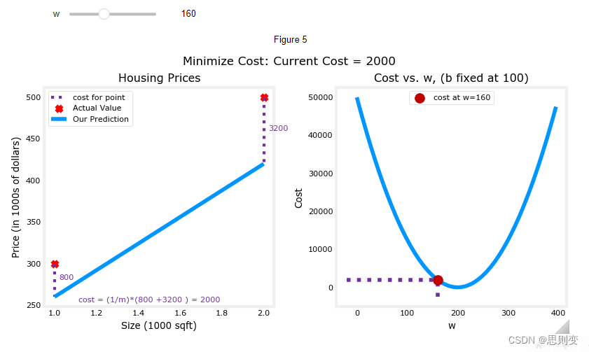
现在假设b=100为固定值,来看一下代价函数和模型精确度的关系:
w=160, 可以看到左图为预测模型,右图为当前w,b组合的情况下的模型的代价函数还没有到达最小值,所以左图中的蓝色预测模型与实际数据的红点并没有重合
w=200,可以看到右图中此时的cost代价函数最小,左图中的实际数据点也与预测模型完全重合

通过上面的对比可以发现通过cost function J(w,b)可以找到最佳的模型参数。因为上面的例子中只有两个训练数据,当有多个训练数据时,所有的训练数据不一定会全落在同一条直线上,这种情况下我们如何寻找cost function J(w,b)=0的参数呢?
下面准备一组数量较多的训练数据:
x_train = np.array([1.0, 1.7, 2.0, 2.5, 3.0, 3.2])
y_train = np.array([250, 300, 480,  430,   630, 730,])


plt.close('all')
fig, ax, dyn_items = plt_stationary(x_train, y_train)
updater = plt_update_onclick(fig, ax, x_train, y_train, dyn_items)
结果为:


上面两张图中第一行右图是cost function 代价函数图,可以看出来多数据的情况下,很有可能是找不到代价函数为0的点的,这时只能寻找最小的点。当代价函数最小的时候,第一行左图中的线性模型与实际数据匹配度较高。
成本函数对损失进行平方的事实确保了“误差面”像汤碗一样凸起。它将始终具有一个最小值,可以通过遵循所有维度的梯度来达到该最小值。在前面的图中,由于w和b维度的比例不同,因此不容易识别。下面的图,其中w和b是对称的,可以发现,上图中的cost 图形,就是下图中这个碗被拍扁的状态。

梯度下降——自动寻找最小的cost function 代价函数
上一部分中代价函数是通过手动来调整的,在实际应用中手动调整是不现实的,因此需要一种方法来自动寻找最小的代价函数。
梯度的概念:
要引入梯度需要先知道方向导数这个东西。方向导数是函数定义域的内点对某一方向求导得到的导数。就是说函数上每一个点都有向各种方向变大变小的趋势,而方向导数就是函数上某一个点朝某一个方向上的导数。而同一个点上朝各个方向的导数大小是不一样的,梯度就是这些导数中变化量最大的那个方向。
具体分析可以参考知乎文章:通俗理解方向导数、梯度|学习笔记 - 知乎 (zhihu.com)
上一张AI大佬的图来直观感受一下梯度:
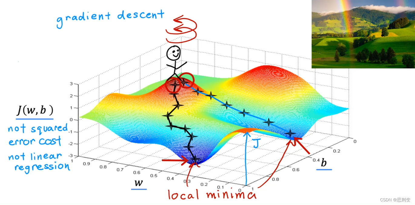
下山的路有很多条,只有沿梯度方向下山最快。因此我们要沿着梯度的方向来快速的寻找cost function的最小值。
梯度下降公式:

实现代码为:
代码实现了上面的公式4和公式5,也就是计算了w,b各自的偏导数。
def compute_gradient(x, y, w, b):
    """
    Computes the gradient for linear regression
    Args:
      x (ndarray (m,)): Data, m examples
      y (ndarray (m,)): target values
      w,b (scalar)    : model parameters
    Returns
      dj_dw (scalar): The gradient of the cost w.r.t. the parameters w
      dj_db (scalar): The gradient of the cost w.r.t. the parameter b
     """

    # Number of training examples
    m = x.shape[0]
    dj_dw = 0
    dj_db = 0

    for i in range(m):
        f_wb = w * x[i] + b
        dj_dw_i = (f_wb - y[i]) * x[i]
        dj_db_i = f_wb - y[i]
        dj_db += dj_db_i
        dj_dw += dj_dw_i
    dj_dw = dj_dw / m
    dj_db = dj_db / m

    return dj_dw, dj_db
现在检验一下这个函数计算出来的是不是梯度:
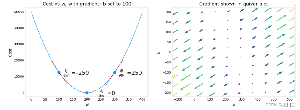
plt_gradients(x_train,y_train, compute_cost, compute_gradient)
plt.show()
结果为:当w=200时,cost function 代价函数的值最小。下面右边的图中,在图的右侧,导数为正数,而在左侧为负数。由于“碗形”,导数将始终导致梯度下降到梯度为零的底部。
上面完成了梯度的计算,现在来进行梯度下降的代码实现:
def gradient_descent(x, y, w_in, b_in, alpha, num_iters, cost_function, gradient_function):
    """
    Performs gradient descent to fit w,b. Updates w,b by taking
    num_iters gradient steps with learning rate alpha

    Args:
      x (ndarray (m,))  : Data, m examples
      y (ndarray (m,))  : target values
      w_in,b_in (scalar): initial values of model parameters
      alpha (float):     Learning rate
      num_iters (int):   number of iterations to run gradient descent
      cost_function:     function to call to produce cost
      gradient_function: function to call to produce gradient

    Returns:
      w (scalar): Updated value of parameter after running gradient descent
      b (scalar): Updated value of parameter after running gradient descent
      J_history (List): History of cost values
      p_history (list): History of parameters [w,b]
      """

    w = copy.deepcopy(w_in)  # avoid modifying global w_in
    # An array to store cost J and w's at each iteration primarily for graphing later
    J_history = []
    p_history = []
    b = b_in
    w = w_in

    for i in range(num_iters):
        # Calculate the gradient and update the parameters using gradient_function
        dj_dw, dj_db = gradient_function(x, y, w, b)

        # Update Parameters using equation (3) above
        b = b - alpha * dj_db
        w = w - alpha * dj_dw

        # Save cost J at each iteration
        if i < 100000:  # prevent resource exhaustion
            J_history.append(cost_function(x, y, w, b))
            p_history.append([w, b])
        # Print cost every at intervals 10 times or as many iterations if < 10
        if i % math.ceil(num_iters / 10) == 0:
            print(f"Iteration {i:4}: Cost {J_history[-1]:0.2e} ",
                  f"dj_dw: {dj_dw: 0.3e}, dj_db: {dj_db: 0.3e}  ",
                  f"w: {w: 0.3e}, b:{b: 0.5e}")

    return w, b, J_history, p_history  # return w and J,w history for graphing
梯度下降的代码已经完成,我们来通过下面的代码使用这个梯度下降算法寻找最优的模型:
寻找最优模型的方法是不断更新w和b直到w,b收敛。那么如何判断收敛呢?
假设初始的模型参数w_init和b_init 都是0,训练次数为10000次,学习率tmp_aplha为1.0e-2也就是0.01。然后打印出最终的参数w和b。
# 目前还是通过多次的迭代更新w,b,来确认最合适的w,b参数。有没可能不手动更新迭代次数,由模型自己寻找最佳参数
# initialize parameters
w_init = 0
b_init = 0
# some gradient descent settings
iteration = 10000
tmp_alpha = 1.0e-2

# run gradient descent
w_final,b_final , J_hist, p_hist = gradient_descent(x_train,y_train,w_init,b_init,tmp_alpha,
                                                  iteration,compute_cost,compute_gradient)

print(f"(w,b) found by gradient descent: ({w_final:8.4f},{b_final:8.4f})")
最终输出为:w=200,b=100
Iteration    0: Cost 7.93e+04  dj_dw: -6.500e+02, dj_db: -4.000e+02   w:  6.500e+00, b: 4.00000e+00
Iteration 1000: Cost 3.41e+00  dj_dw: -3.712e-01, dj_db:  6.007e-01   w:  1.949e+02, b: 1.08228e+02
Iteration 2000: Cost 7.93e-01  dj_dw: -1.789e-01, dj_db:  2.895e-01   w:  1.975e+02, b: 1.03966e+02
Iteration 3000: Cost 1.84e-01  dj_dw: -8.625e-02, dj_db:  1.396e-01   w:  1.988e+02, b: 1.01912e+02
Iteration 4000: Cost 4.28e-02  dj_dw: -4.158e-02, dj_db:  6.727e-02   w:  1.994e+02, b: 1.00922e+02
Iteration 5000: Cost 9.95e-03  dj_dw: -2.004e-02, dj_db:  3.243e-02   w:  1.997e+02, b: 1.00444e+02
Iteration 6000: Cost 2.31e-03  dj_dw: -9.660e-03, dj_db:  1.563e-02   w:  1.999e+02, b: 1.00214e+02
Iteration 7000: Cost 5.37e-04  dj_dw: -4.657e-03, dj_db:  7.535e-03   w:  1.999e+02, b: 1.00103e+02
Iteration 8000: Cost 1.25e-04  dj_dw: -2.245e-03, dj_db:  3.632e-03   w:  2.000e+02, b: 1.00050e+02
Iteration 9000: Cost 2.90e-05  dj_dw: -1.082e-03, dj_db:  1.751e-03   w:  2.000e+02, b: 1.00024e+02
(w,b) found by gradient descent: (199.9929,100.0116)
上面可以尝试迭代次数不同的情况下,得出的w和b是不一样的。目前还是通过手更新迭代次数来寻找w,b,有没有可能不需要人的干预就能实现模型自己学习,自己寻找最佳的w,b组合,后面的CNN应该能做到这一点。
至此,线性模型的实现,模型性能的衡量参数,模型最佳参数的训练方法基本就整理清楚了。