简介

用户有时需要根据期刊的配图绘制要求进行诸如字体、刻度轴、轴脊、图例等图层属性的定制化修改，耗时的同时也会容易导致用户忽略一些图层细节要求。

SciencePlots 作为一个专门用于科研论文绘图的第三方拓展工具包，提供了主流英文科技期刊（如 Nature、Science 和 IEEE 等）的 Matplotlib 图样式（Matplotlib Styles）。

SciencePlots 的安装代码如下：

pip install SciencePlots

安装 LaTeX

为了更好地显示学术论文插图和方便后续印刷，插图中的字体样式一般要求为 LaTeX 编写样式，SciencePlots 可以简单地实现该要求。SciencePlots 库实现 LaTeX 编写样式需要使用者在计算机上安装 LaTeX。

其余类型操作系统安装步骤参考 SciencePlots 官方教程即可。

安装 MikTex 和 Ghostscript
ScienePlots 库官方建议用户使用 MikTex 软件安装 LaTeX，用户直接从 MikTex 官网下载其最新版本并安装即可。Ghostscript 是一套建基于 Adobe、PostScript 及可移植文档格式（PDF）的页面描述语言等而编译成的免费软件，用户可从其官网下载最新版本并安装。
将软件的安装路径添加到系统环境变量中
在安装了上述两款软件后，用户还需要将它们的安装路径添加到系统环境变量中，具体为“\...\miktex\bin\x64”和“\...\gs__( 版本号)\bin”。添加完系统环境变量后，重启，相关配置即可生效。

SciencePlots 绘图示例

如果读者投稿的期刊有特殊字体要求，那么读者可设置不使用 LaTeX 绘图：：plt.style.use(['science',' no-latex'])。

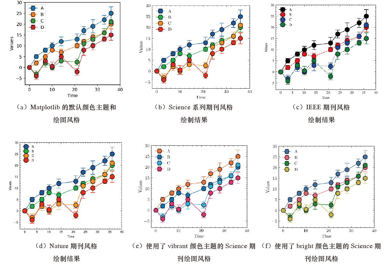
下图为 SciencePlots 中多种绘图风格示例，
（a）为 Matplotlib 的默认颜色主题和绘图风格

import pandas as pd
import numpy as np
import matplotlib.pyplot as plt


data = pd.read_excel(r"\分组误差线图构建.xlsx")

#(a)Matplotlib的默认颜色主题和绘图风格
selsect = ["A","B","C","D"]
colors = ["#2FBE8F","#459DFF","#FF5B9B","#FFCC37"]
fig,ax = plt.subplots(figsize=(4,3.5),dpi=100,facecolor="w")

for index,color in zip(selsect,colors):
    data_selcet = data.loc[data['type']==index,:]
    ax.errorbar(x=data_selcet["time"],y=data_selcet["mean"],yerr=data_selcet["sd"],
                linewidth=1,marker='o',ms=10,mew=1,mec='k',capsize=5,label=index)
    ax.legend()
    ax.set(xlabel='Time', ylabel='Values',
           xlim=(-2,40),ylim=(-8,30))

plt.savefig('\第2章 绘制工具及其重要特征\图2-3-8 ScienecePlots_matplotlib.png', 
         bbox_inches='tight',dpi=600)
plt.savefig('\第2章 绘制工具及其重要特征\图2-3-8 ScienecePlots_matplotlib.pdf', 
         bbox_inches='tight') 
plt.show()

（b）为 Science 系列期刊风格绘制结果

#(b)Science系列期刊风格绘制结果

selsect = ["A","B","C","D"]
colors = ["#2FBE8F","#459DFF","#FF5B9B","#FFCC37"]
plt.style.use('science')
fig,ax = plt.subplots(figsize=(4,3.5),dpi=100,facecolor="w")
for index,color in zip(selsect,colors):
    data_selcet = data.loc[data['type']==index,:]
    ax.errorbar(x=data_selcet["time"],y=data_selcet["mean"],yerr=data_selcet["sd"],
                linewidth=1,marker='o',ms=10,mew=1,mec='k',capsize=5,label=index)
    ax.legend()
    ax.set(xlabel='Time', ylabel='Values',
           xlim=(-2,40),ylim=(-8,30))
plt.savefig('\第2章 绘制工具及其重要特征\图2-3-8 SciencePlots_science.png', 
         bbox_inches='tight',dpi=600)
plt.savefig('\第2章 绘制工具及其重要特征\图2-3-8 SciencePlots_science.pdf', 
         bbox_inches='tight') 
plt.show()

（c）为 IEEE 期刊风格绘制结果

#(c)IEEE期刊风格绘制结果
selsect = ["A","B","C","D"]
colors = ["#2FBE8F","#459DFF","#FF5B9B","#FFCC37"]
plt.style.use(['science','ieee'])
fig,ax = plt.subplots(figsize=(4,3.5),dpi=100,facecolor="w")
for index,color in zip(selsect,colors):
    data_selcet = data.loc[data['type']==index,:]
    ax.errorbar(x=data_selcet["time"],y=data_selcet["mean"],yerr=data_selcet["sd"],
                linewidth=1,marker='o',ms=10,mew=1,mec='k',capsize=5,label=index)
    ax.legend()
    ax.set(xlabel='Time', ylabel='Values',
           xlim=(-2,40),ylim=(-8,30))
plt.savefig('\第2章 绘制工具及其重要特征\图2-3-8 SciencePlots_ieee.png', 
         bbox_inches='tight',dpi=600)
plt.savefig('\第2章 绘制工具及其重要特征\图2-3-8 SciencePlots_ieee.pdf', 
         bbox_inches='tight') 
plt.show()

（d）为 Nature 期刊风格绘制结果

#(d)Nature期刊风格绘制结果
colors = ["#2FBE8F","#459DFF","#FF5B9B","#FFCC37"]
selsect = ["A","B","C","D"]
plt.style.use(['science','nature'])
fig,ax = plt.subplots(figsize=(4,3.5),dpi=100,facecolor="w")
for index,color in zip(selsect,colors):
    data_selcet = data.loc[data['type']==index,:]
    ax.errorbar(x=data_selcet["time"],y=data_selcet["mean"],yerr=data_selcet["sd"],
                linewidth=1,marker='o',ms=10,mew=1,mec='k',capsize=5,label=index)
    ax.legend()
    ax.set(xlabel='Time', ylabel='Values',
           xlim=(-2,40),ylim=(-8,30))

plt.savefig('\第2章 绘制工具及其重要特征\图2-3-8 SciencePlots_nature.png', 
         bbox_inches='tight',dpi=600)
plt.savefig('\第2章 绘制工具及其重要特征\图2-3-8 SciencePlots_nature.pdf', 
         bbox_inches='tight') 
plt.show()

（e）为使用了 vibrant 颜色主题的 Science 期刊绘图风格

#(e)使用了vibrant 颜色主题的Science期刊绘图风格
selsect = ["A","B","C","D"]
plt.style.use(['science','vibrant'])
fig,ax = plt.subplots(figsize=(4,3.5),dpi=100,facecolor="w")
for index,color in zip(selsect,colors):
    data_selcet = data.loc[data['type']==index,:]
    ax.errorbar(x=data_selcet["time"],y=data_selcet["mean"],yerr=data_selcet["sd"],
                linewidth=1,marker='o',ms=10,mew=1,mec='k',capsize=5,label=index)
    ax.legend()
    ax.set(xlabel='Time', ylabel='Values',
           xlim=(-2,40),ylim=(-8,30))

plt.savefig('\第2章 绘制工具及其重要特征\图2-3-8 SciencePlots_vibrant.png', 
         bbox_inches='tight',dpi=600)
plt.savefig('\第2章 绘制工具及其重要特征\图2-3-8 SciencePlots_vibrant.pdf', 
         bbox_inches='tight') 
plt.show()

（f）为使用了 bright 颜色主题的 Science 期刊绘图风格

#(f)使用了bright颜色主题的Science期刊绘图风格
selsect = ["A","B","C","D"]
plt.style.use(['science','bright'])
fig,ax = plt.subplots(figsize=(4,3.5),dpi=100,facecolor="w")
for index,color in zip(selsect,colors):
    data_selcet = data.loc[data['type']==index,:]
    ax.errorbar(x=data_selcet["time"],y=data_selcet["mean"],yerr=data_selcet["sd"],
                linewidth=1,marker='o',ms=10,mew=1,mec='k',capsize=5,label=index)
    ax.legend()
    ax.set(xlabel='Time', ylabel='Values',
           xlim=(-2,40),ylim=(-8,30))
           
plt.savefig('\第2章 绘制工具及其重要特征\图2-3-8 SciencePlots_bright.png', 
         bbox_inches='tight',dpi=600)
plt.savefig('\第2章 绘制工具及其重要特征\图2-3-8 SciencePlots_bright.pdf', 
         bbox_inches='tight') 
plt.show()

更多绘图风格参考 SciencePlots 官网。

提示：SciencePlots 库不但提供了主流英文科技期刊的绘图风格模板，而且能够实现不同绘图风格的混合使用。此外，在使用该库的绘图风格时，读者可通过plt.style.use('science') 设置全局绘图风格，也可通过以下语句来临时使用绘图风格。

with plt.style.context('science '):
	plt.figure()
	plt.plot(x,y)
	plt.show()

建议使用全局设置，因为在使用临时绘图风格，特别是使用了 LaTeX 字符时，将导致绘制图例、轴标签等图层属性时，无法使用 LaTeX 字符风格，造成绘图结果整体不协调问题。引入 SciencePlots 绘图主题样式的方式可能会随着版本的更新有所不同，读者应查看 SciencePlots 官网，使用其最新的引入方式。

参考书籍：宁海涛.科研论文配图绘制指南——基于Python[M].北京：人民邮电出版社，2023：42-44.

SciencePlots 基本语法及特点

文章目录

简介

安装 LaTeX

SciencePlots 绘图示例

猜你喜欢