简介
科研论文配图多图层元素(字体、坐标轴、图例等)的绘制条件提出了更高要求,我们需要更改 Matplotlib 和 Seaborn 中的多个绘制参数,特别是在绘制含有多个子图的复杂图形时,容易造成绘制代码冗长。
作为一个简洁的 Matplotlib 包装器,ProPlot 库是 Matplotlib 面向对象绘图方法(object-oriented interface)的高级封装,整合了 cartopy/Basemap 地图库、xarray 和 pandas,可弥补 Matplotlib 的部分缺陷。ProPlot 可以让 Matplotlib 爱好者拥有更加顺滑的绘图体验。
多子图绘制处理
共享轴标签
在使用 Matplotlib 绘制多子图时,不可避免地要进行轴刻度标签、轴标签、颜色条(colorbar)和图例的重复绘制操作,导致绘图代码冗长。此外,我们还需要为每个子图添加顺序标签(如 a、b、c 等)。ProPlot 可以直接通过其内置方法来绘制不同样式的子图标签,而 Matplotlib 则需要通过自定义函数进行绘制。
ProPlot 中的 figure () 函数的 sharex、sharey、share 参数可用于控制不同的轴标签样式,它们的可选值及说明如下:

下面是使用 ProPlot 绘制的多子图轴标签共享示意图,其中
- (a)为无共享轴标签样式;
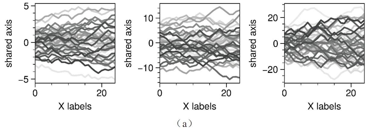
- (b)为设置 Y 轴共享标签样式;
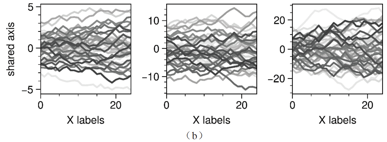
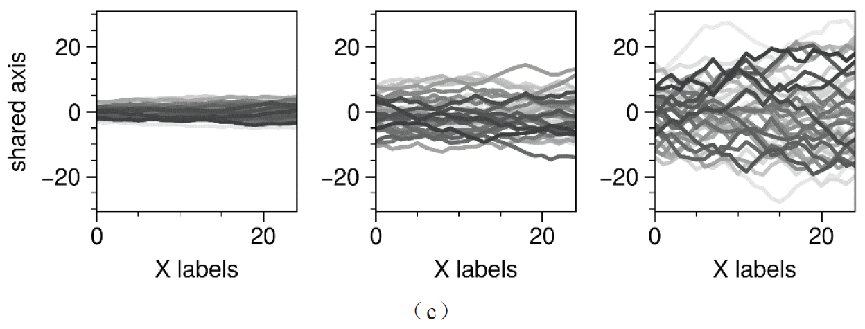
- (c)展示了设置 Y 轴共享方式为 Limits 时的样式,可以看出,每个子图的刻度范围被强制设置为相同,导致有些子图显示不全;
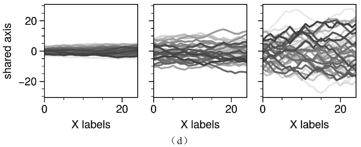
- (d)展示了设置 Y 轴共享方式为 True 时的样式,此时,轴标签、刻度标签都实现了共享。
import pandas as pd
import numpy as np
import proplot as pplt
import matplotlib.pyplot as plt

N = 50
M = 40
state = np.random.RandomState(51423)
cycle = pplt.Cycle('grays', M, left=0.1, right=0.8)

datas = []
for scale in (1, 3, 7, 0.2):
    data = scale * (state.rand(N, M) - 0.5).cumsum(axis=0)[N // 2:, :]
    datas.append(data)

# Plots with different sharing and spanning settings
# Note that span=True and share=True are the defaults
spans = (False, False, False, False)
shares = (False, 'labels', 'limits', True)
for i, (span, share) in enumerate(zip(spans, shares)):
	# note: there is sharey
    fig = pplt.figure(refaspect=1, refwidth=1.06, spanx=span, sharey=share)
    axs = fig.subplots(ncols=3)
    for ax, data in zip(axs, datas):
        on = ('off', 'on')[int(span)]
        ax.plot(data, cycle=cycle)
        ax.format(
            grid=False, xlabel='X labels', ylabel='shared axis',
            #suptitle=f'Sharing mode {share!r} (level {i}) with spanning labels {on}'
        )
        fig.save(r'\第2章 绘制工具及其重要特征\Proplot_subplot_share'+str(share)+'.png', bbox_inches='tight',dpi=600)
        fig.save(r'\第2章 绘制工具及其重要特征\\Proplot_subplot_share'+str(share)+'.pdf', bbox_inches='tight')

plt.show()
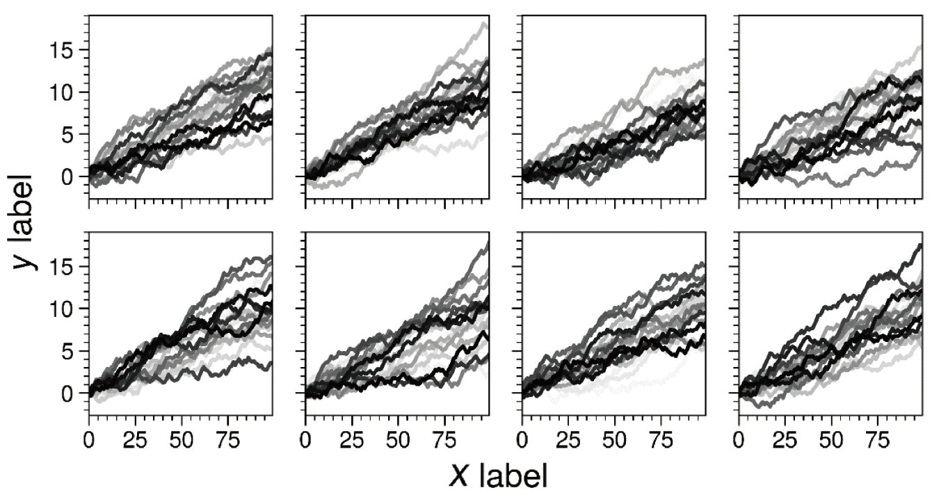
“跨度”轴标签
figure() 函数中的 spanx、spany 和 span 参数用于控制是否对 X 轴、Y 轴或两个轴使用“跨度”轴标签,即当多个子图的 X 轴、Y 轴标签相同时,使用一个轴标签替代即可。
import pandas as pd
import numpy as np
import proplot as pplt
import matplotlib.pyplot as plt


state = np.random.RandomState(51423)

# Plots with minimum and maximum sharing settings
# Note that all x and y axis limits and ticks are identical
spans = (True, True)
shares = (True, 'all')
titles = ('Minimum sharing', 'Maximum sharing')
for span, share, title in zip(spans, shares, titles):
    fig = pplt.figure(refwidth=1, span=span, share=share)
    axs = fig.subplots(nrows=2, ncols=4)
    for ax in axs:
        data = (state.rand(100, 20) - 0.4).cumsum(axis=0)
        ax.plot(data, cycle='grays')
    axs.format(
        xlabel='xlabel', ylabel='ylabel',
        grid=False, xticks=25, yticks=5,labelsize=13
    )
fig.save(r'\第2章 绘制工具及其重要特征\图2-3-2 Proplot_subplot_span.png',
         bbox_inches='tight',dpi=600)
fig.save(r'\第2章 绘制工具及其重要特征\图2-3-2 Proplot_subplot_span.pdf',
         bbox_inches='tight')


plt.show()
多子图序号的绘制
在科研论文配图中存在多个子图的情况下,一项工作是对每个子图进行序号标注。ProPlot 库为绘图对象(figure.Figure 和 axes.Axes)提供了灵活的 format () 方法,该方法可用于绘制不同的子图序号样式和位置。
format() 函数中的位置参数(abcloc)的可选值如下:
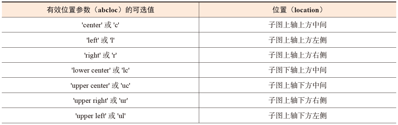


其中,子图序号 G ~ I 添加了背景边框,这是通过将 format () 函数的参数 abcbbox 设置为 True 实现的。此外,参数 abcborder、abc_kw 和 abctitlepad 分别用于控制子图序号的文本边框、文本属性(颜色、粗细等)、子图序号与子图标题间距属性。
import pandas as pd
import numpy as np
import proplot as pplt
import matplotlib.pyplot as plt


fig = pplt.figure(figsize=(8,5.5),space=1, refwidth='10em')
axs = fig.subplots(nrows=3, ncols=3)
locs = ("c","l","r","lc","uc","ur","ul","ll","lr")
abcs = ("a","a.","(a)","[a]","(a","A","A.","(A)","(A.)")
axs.format(abcsize=16,xlabel='x axis', ylabel='y axis',labelsize=18)
axs[-3:].format(abcbbox=True)
axs[0, 0].format(abc="a", abcloc="c",abcborder=True)
axs[0, 1].format(abc="a.", abcloc="l")
axs[0, 2].format(abc="(a)", abcloc="r")
axs[1, 0].format(abc="[a]", abcloc="lc",facecolor='gray5')
axs[1, 1].format(abc="(a", abcloc="uc",facecolor='gray5')
axs[1, 2].format(abc="A", abcloc="ur",facecolor='gray5')
axs[2, 0].format(abc="A.", abcloc="ul",)
axs[2, 1].format(abc="(A)", abcloc="ll")
axs[2, 2].format(abc="(A.)", abcloc="lr")
fig.save(r'\第2章 绘制工具及其重要特征\\图2-3-3 Proplot_abc.png',
         bbox_inches='tight',dpi=600)
fig.save(r'\第2章 绘制工具及其重要特征\\图2-3-3 Proplot_abc.pdf',
         bbox_inches='tight')
plt.show()
更多关于子图属性的添加和修改示例见 ProPlot 官方教程。
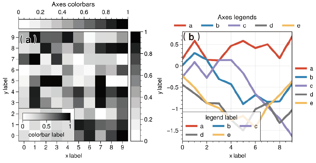
更简单的颜色条和图例
在使用 Matplotlib 的过程中,在子图外部绘制图例有时比较麻烦。通常,我们需要手动定位图例并调整图形和图例之间的间距,为图例在绘图对象中腾出绘制空间。此外,在子图外部绘制颜色条(colorbar)时,如
fig.colorbar (..., ax=ax),需要从父图中借用部分空间,这可能导致具有多个子图的图形对象的显示出现不对称问题。而在 Matplotlib 中,绘制插入绘图对象内部的颜色条和生成宽度一致的子图外部颜色条通常也很困难,因为插入的颜色条会过宽或过窄,与整个子图存在比例不协调等问题。
colorbar 即主图旁一个长条状的小图,能够辅助表示主图中colormap 的颜色组成和颜色与数值的对应关系。
ProPlot 库中有一个专门用于绘制单个子图或多个连续子图的颜色条和图例的简单框架,该框架将位置参数传递给 ProPlot 的 axes.Axes.colorbar 或 axes.Axes.legend,完成特定子图不同位置颜色条或图例的绘制。
import pandas as pd
import numpy as np
import proplot as pplt
import matplotlib.pyplot as plt

fig = pplt.figure(share=False, refwidth=2.3)

# Colorbars
ax = fig.subplot(121)
state = np.random.RandomState(51423)
m = ax.heatmap(state.rand(10, 10), colorbar='t', cmap='grays')
ax.colorbar(m, loc='r')
ax.colorbar(m, loc='ll', label='colorbar label')
ax.format(title='Axes colorbars')

# Legends
ax = fig.subplot(122)
ax.format(title='Axes legends', titlepad='0em')
hs = ax.plot(
    (state.rand(10, 5) - 0.5).cumsum(axis=0), linewidth=3,
    cycle='ggplot', legend='t',
    labels=list('abcde'), legend_kw={

    'ncols': 5, 'frame': False}
)
ax.legend(hs, loc='r', ncols=1, frame=False)
ax.legend(hs, loc='ll', label='legend label')
fig.format(abc="(a)", abcloc="ul",abcsize=15,
           xlabel='xlabel', ylabel='ylabel')

fig.save('\第2章 绘制工具及其重要特征\图2-3-4 Proplot_axes_cb_legend.png',
         bbox_inches='tight',dpi=600)
fig.save('\第2章 绘制工具及其重要特征\图2-3-4 Proplot_axes_cb_legend.pdf',
         bbox_inches='tight')
plt.show()
想要沿图形边缘绘制颜色条或图例,使用 proplot.figure.Figure.colorbar 和 proplot.figure.Figure.legend 即可。

import pandas as pd
import numpy as np
import proplot as pplt
import matplotlib.pyplot as plt


state = np.random.RandomState(51423)
fig, axs = pplt.subplots(
    ncols=2, nrows=2, order='F', refwidth=1.7, wspace=2.5, share=False
)

# Plot data
data = (state.rand(50, 50) - 0.1).cumsum(axis=0)
for ax in axs[:2]:
    m = ax.contourf(data, cmap='grays', extend='both')
hs = []
colors = pplt.get_colors('grays', 5)
for abc, color in zip('ABCDEF', colors):
    data = state.rand(10)
    for ax in axs[2:]:
        h, = ax.plot(data, color=color, lw=3, label=f'line {

      abc}')
    hs.append(h)

# Add colorbars and legends
fig.colorbar(m, length=0.8, label='colorbar label', loc='b', col=1, locator=5)
fig.colorbar(m, label='colorbar label', loc='l')
fig.legend(hs, ncols=2, center=True, frame=False, loc='b', col=2)
fig.legend(hs, ncols=1, label='legend label', frame=False, loc='r')
fig.format(abc='A', abcloc='ul')
for ax, title in zip(axs, ('2D {} #1', '2D {} #2', 'Line {} #1', 'Line {} #2')):
    ax.format(xlabel='xlabel', title=title.format('dataset'))

fig.save(r'\第2章 绘制工具及其重要特征\Proplot_figure_cb_legend.png',
         bbox_inches='tight',dpi=600)
fig.save(r'\第2章 绘制工具及其重要特征\Proplot_figure_cb_legend.pdf',
         bbox_inches='tight')
plt.show()
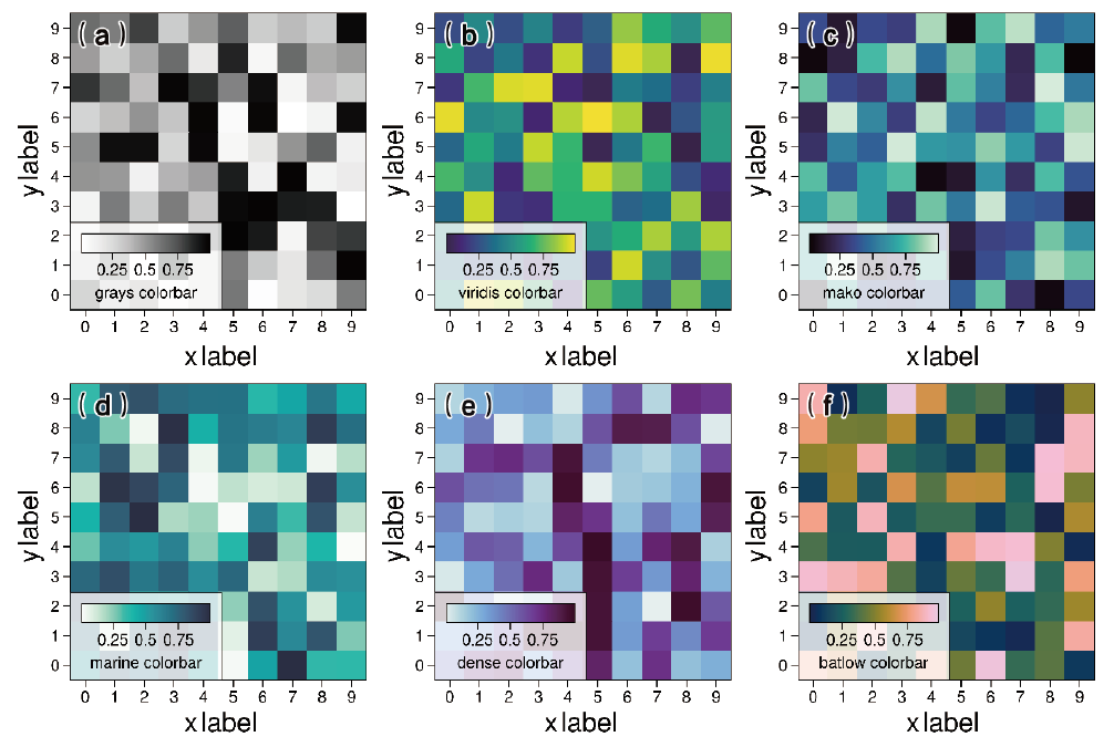
更加美观的颜色和字体
科学可视化展示中的一个常见问题是使用像“jet”这样的存在误导的颜色映射(colormap)去映射对应数值,这种颜色映射在色相、饱和度和亮度上都存在明显的视觉缺陷。Matplotlib 中可供选择的颜色映射选项较少,仅存在几个色相相似的颜色映射,无法应对较复杂的数值映射场景。
ProPlot 库封装了大量的颜色映射选项,不但提供了来自 Seaborn、cmOcean、SciVisColor 等的拓展包和 Scientific colour maps 等项目中的多个颜色映射选项,而且定义了一些默认颜色选项和一个用于生成新颜色条的 PerceptualColormap 类。
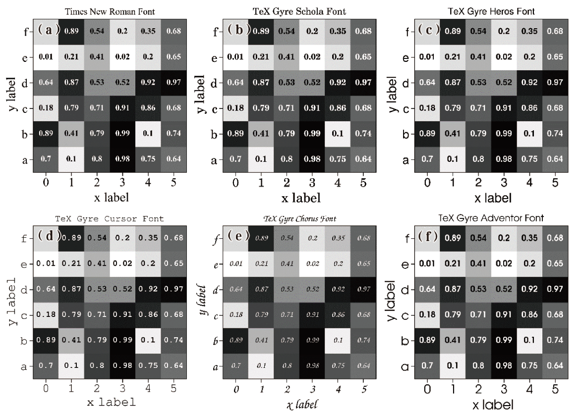
Matplotlib 的默认绘图字体为 DejaVu Sans,这种字体是开源的,但是,从美学角度来说,它并不太讨人喜欢。ProPlot 库还附带了其他几种无衬线字体和整个 TeX Gyre 字体系列,这些字体更加符合一些科技期刊对科研论文配图的绘制要求。
下面为使用 ProPlot 的不同颜色映射选项绘制的不同颜色映射的效果图。
(a)为灰色(grays)系颜色映射
(b)为 Matplotlib 默认的 viridis 颜色映射
(c)为 Seaborn 中的 mako 颜色映射
(d)为 ProPlot 中的 marine 颜色映射
(e)为 cmOcean 中的 dense 颜色映射
(f)为 Scientific colour maps 中的 batlow 颜色映射。
import pandas as pd
import numpy as np
import proplot as pplt
import matplotlib.pyplot as plt


fig = pplt.figure(share=False, refwidth=2.3)

# Colorbars
ax = fig.subplot(231)
state = np.random.RandomState(51423)
data = 1 + (state.rand(12, 10) - 0.45).cumsum(axis=0)
m = ax.heatmap(state.rand(10, 10), cmap='grays')
ax.colorbar(m, loc='ll', label='grays colorbar')
ax = fig.subplot(232)
m = ax.heatmap(state.rand(10, 10), cmap='viridis')
ax.colorbar(m, loc='ll', label='viridis colorbar')

ax = fig.subplot(233)
m = ax.heatmap(state.rand(10, 10), cmap='mako')
ax.colorbar(m, loc='ll', label='mako colorbar')

ax = fig.subplot(234)
m = ax.heatmap(state.rand(10, 10), cmap='marine')
ax.colorbar(m, loc='ll', label='marine colorbar')

ax = fig.subplot(235)
m = ax.heatmap(state.rand(10, 10), cmap='dense')
ax.colorbar(m, loc='ll', label='dense colorbar')

ax = fig.subplot(236)
m = ax.heatmap(state.rand(10, 10), cmap='batlow')
ax.colorbar(m, loc='ll', label='batlow colorbar')

fig.format(abc="(a)", abcloc="ul",abcsize=15,
           xlabel='xlabel', ylabel='ylabel',labelsize=15)

fig.save(r'\第2章 绘制工具及其重要特征\图2-3-6 Proplot_colormaps.png',
         bbox_inches='tight',dpi=600)
fig.save(r'\第2章 绘制工具及其重要特征\图2-3-6 Proplot_colormaps.pdf',
         bbox_inches='tight')
plt.show()
更多颜色映射的绘制请参考 ProPlot 官方教程。
下面是 ProPlot 中部分字体绘制的可视化结果,其中(a)(b)(c)中展示的 3 种字体是科研论文配图绘制中的常用字体。
import pandas as pd
import numpy as np
import proplot as pplt
import matplotlib.pyplot as plt
from proplot import rc

# Sample data
state = np.random.RandomState(51423)
data = state.rand(6, 6)
data = pd.DataFrame(data, index=pd.Index(['a', 'b', 'c', 'd', 'e', 'f']))

fig = pplt.figure(share=False, refwidth=2.3)
# 参数 rc 则用于覆盖预设样式字典中的值的参数映射,只更新样式中的一部分参数。
rc["font.family"] = "Times New Roman"
ax = fig.subplot(231)
m = ax.heatmap(
    data, cmap='grays',
    labels=True, precision=2, labels_kw={

    'weight': 'bold'}
)
ax.format(title='Times New Roman Font')

rc["font.family"] = "TeX Gyre Schola"
ax = fig.subplot(232)
m = ax.heatmap(
    data, cmap='grays',
    labels=True, precision=2, labels_kw={

    'weight': 'bold'}
)
ax.format(title='TeX Gyre Schola Font')

rc["font.family"] = "TeX Gyre Heros"
ax = fig.subplot(233)
m = ax.heatmap(
    data, cmap='grays',
    labels=True, precision=2, labels_kw={

    'weight': 'bold'}
)
ax.format(title='TeX Gyre Heros Font')

rc["font.family"] = "TeX Gyre Cursor"
ax = fig.subplot(234)
m = ax.heatmap(
    data, cmap='grays',
    labels=True, precision=2, labels_kw={

    'weight': 'bold'}
)
ax.format(title='TeX Gyre Cursor Font')

rc["font.family"] = "TeX Gyre Chorus"
ax = fig.subplot(235)
m = ax.heatmap(
    data, cmap='grays',
    labels=True, precision=2, labels_kw={

    'weight': 'bold'}
)
ax.format(title='TeX Gyre Chorus Font')

rc["font.family"] = "TeX Gyre Adventor"
ax = fig.subplot(236)
m = ax.heatmap(
    data, cmap='grays',
    labels=True, precision=2, labels_kw={

    'weight': 'bold'}
)
ax.format(title='TeX Gyre Adventor Font')

fig.format(abc="(a)", abcloc="ul",abcsize=15,
           xlabel='xlabel', ylabel='ylabel',labelsize=14)


fig.save(r'\第2章 绘制工具及其重要特征\图2-3-7 Proplot_fonts.png',
         bbox_inches='tight',dpi=600)
fig.save(r'\第2章 绘制工具及其重要特征\图2-3-7 Proplot_fonts.pdf',
         bbox_inches='tight')
plt.show()
ProPlot 绘图工具库为基于 Python 基础绘图工具 Matplotlib 的第三方优质拓展库,既可使用它自身的绘图函数绘制不同类型的图,也可仅使用其优质的绘图主题,即导入 ProPlot 库。
以上代码基于 ProPlot 0.9.5 版本,不包括 Matplotlib 3.4.3 的后续版本的升级优化部分。ProPlot 0.9.5 版本不支持 Matplotlib 3.5 系列版本。想要使用 ProPlot 绘制不同需求的图形结果或使用 ProPlot 优质学术风格绘图主题,可自行安装 Matplotlib 3.4 系列版本。