AI quantitative model prediction

Quantitative finance has been in foreign countries for decades, but it has emerged in China for less than a decade. This is a very challenging area. Quantitative finance combines the essence of mathematical statistics, financial theory, sociology, psychology and other disciplines, and pays special attention to practice. Due to the diversity of individuals involved in the market game and the complexity of group effects, quantitative finance is characterized by great challenges and great opportunities. This competition uses the methods and tools of big data and machine learning to understand the principles of market behavior, create quantitative strategies through data analysis and models, use historical data to verify the effectiveness of quantitative strategies, and conduct evaluation through real-time data.

Given data set: Given training set (including validation set), including 10 (non-public) stocks, 79 trading days of L1snapshot data (the first 64 trading days are training data, for training purposes; The last 15 trading days are test data, which cannot be used for training. The data has been normalized and hidden, including 5 files of volume/price, middle price, trading volume and other data (please refer to the follow-up data description for details).

Forecasting task: Using past and current data to predict the moving direction of the future central parity, model training and forecasting on the data

Enter data:

Market frequency: 3 seconds a data point (also known as 1 tick snapshot);

Each data point includes the current latest transaction price/fifth volume price/transaction amount in the past 3 seconds;

Each data point in the training set contains 5 prediction labels; Allows you to use data of no more than 100 ticks in the past (including the current tick) to predict the direction of the midpoint movement after N ticks in the future.

Prediction time span: 5, 10, 20, 40, 60 ticks, 5 prediction tasks;

That is, after t+5tick, t+10tick, t+20tick, t+40tick, t+60tick are respectively predicted at time t: the latest midprice is compared with the midprice at time t: down/unchanged/up.

Contest data set
Market frequency: 3 seconds a data point (also known as 1 tick snapshot);
Each data point includes the current latest transaction price/fifth volume price/transaction amount in the past 3 seconds;
Each data point in the training set contains 5 prediction labels; Allows you to use data of no more than 100 ticks in the past (including the current tick) to predict the direction of the midpoint movement after N ticks in the future.
Prediction time span: 5, 10, 20, 40, 60 ticks, 5 prediction tasks; That is, after t+5tick, t+10tick, t+20tick, t+40tick, t+60tick are respectively predicted at time t: the latest midprice is compared with the midprice at time t: down/unchanged/up.

Evaluation index
Based on the submitted result file, macro-F1 score is used to evaluate the model, and the highest score among label_5, label_10, label_20, label_40 and label_60 is taken as the final score.

Solution idea
The task is to build an AI quantitative model that uses past and current data to predict the direction of future midpoint movements. This AI quantification task is a typical time series regression prediction problem. To deal with this problem, it is generally recommended to use machine learning methods, such as CatBoost, LightGBM, XGBoost and other tree models, which can better handle numerical data and have high interpretability. Or the deep learning method is used, but the construction of the deep model is complicated, and the model structure needs to be constructed by itself. The numerical data needs to be standardized, and the interpretability is weak. When we solve machine learning problems, we generally follow the following process:

 In this Baseline, we use the CatBoost model of machine learning to solve this problem, and will lead you to run through the entire competition practice process of data exploration, feature engineering, model training, model validation, and result output.

3.2.1 导入模块

导入我们本次Baseline代码所需的模块（直接用本项目可全部跑通，如希望尝试本地，参考附录 - 实践环境配置）

# 解压数据集，更新所需依赖包

_ = !unzip -qo data/data233139/AI量化模型预测挑战赛公开数据.zip
_ = !pip install --upgrade catboost xgboost lightgbm

import numpy as np
import pandas as pd
from catboost import CatBoostClassifier
from sklearn.model_selection import StratifiedKFold, KFold, GroupKFold
from sklearn.metrics import accuracy_score, f1_score, roc_auc_score, log_loss, mean_squared_log_error
import tqdm, sys, os, gc, argparse, warnings
import matplotlib.pyplot as plt
warnings.filterwarnings('ignore')

3.2.2 数据探索

数据探索性分析，是通过了解数据集，了解变量间的相互关系以及变量与预测值之间的关系，从而帮助我们后期更好地进行特征工程和建立模型，是机器学习中十分重要的一步。

# 读取数据
path = 'AI量化模型预测挑战赛公开数据/'

train_files = os.listdir(path+'train')
train_df = pd.DataFrame()
for filename in tqdm.tqdm(train_files):
    tmp = pd.read_csv(path+'train/'+filename)
    tmp['file'] = filename
    train_df = pd.concat([train_df, tmp], axis=0, ignore_index=True)

test_files = os.listdir(path+'test')
test_df = pd.DataFrame()
for filename in tqdm.tqdm(test_files):
    tmp = pd.read_csv(path+'test/'+filename)
    tmp['file'] = filename
    test_df = pd.concat([test_df, tmp], axis=0, ignore_index=True)

100%|██████████| 1225/1225 [04:26<00:00,  4.59it/s]
100%|██████████| 296/296 [00:14<00:00, 20.00it/s]

首先可以对买价卖价进行可视化分析

选择任意一个股票数据进行可视化分析，观察买价和卖价的关系。下面是对买价和卖价的简单介绍：

• 买价指的是买方愿意为一项股票/资产支付的最高价格。
• 卖价指的是卖方愿意接受的一项股票/资产的最低价格。
• 这两个价格之间的差异被称为点差；点差越小，该品种的流动性越高。

cols = ['n_bid1','n_bid2','n_ask1','n_ask2']
tmp_df = train_df[train_df['file']=='snapshot_sym7_date22_pm.csv'].reset_index(drop=True)[-500:]
tmp_df = tmp_df.reset_index(drop=True).reset_index()
for num, col in enumerate(cols):
    plt.figure(figsize=(20,5))
   
    plt.subplot(4,1,num+1)
    plt.plot(tmp_df['index'],tmp_df[col])
    plt.title(col)
plt.show()
plt.figure(figsize=(20,5))

for num, col in enumerate(cols):
    plt.plot(tmp_df['index'],tmp_df[col],label=col)
plt.legend(fontsize=12)

<Figure size 2000x500 with 1 Axes>

<Figure size 2000x500 with 1 Axes>

<Figure size 2000x500 with 1 Axes>

<Figure size 2000x500 with 1 Axes>

<matplotlib.legend.Legend at 0x7f16327b7400>

<Figure size 2000x500 with 1 Axes>

加上中间价继续可视化，中间价即买价与卖价的均值，数据中有直接给到，我们也可以自己计算。

plt.figure(figsize=(20,5))

for num, col in enumerate(cols):
    
    plt.plot(tmp_df['index'],tmp_df[col],label=col)
    
plt.plot(tmp_df['index'],tmp_df['n_midprice'],label="n_midprice",lw=10)
plt.legend(fontsize=12)

<matplotlib.legend.Legend at 0x7f16305dd0c0>

<Figure size 2000x500 with 1 Axes>

波动率是给定股票价格变化的重要统计指标，因此要计算价格变化，我们首先需要在固定间隔进行股票估值。我们将使用已提供的数据的加权平均价格（WAP）进行可视化，WAP的变化反映股票波动情况。

train_df['wap1'] = (train_df['n_bid1']*train_df['n_bsize1'] + train_df['n_ask1']*train_df['n_asize1'])/(train_df['n_bsize1'] + train_df['n_asize1'])
test_df['wap1'] = (test_df['n_bid1']*test_df['n_bsize1'] + test_df['n_ask1']*test_df['n_asize1'])/(test_df['n_bsize1'] + test_df['n_asize1'])

tmp_df = train_df[train_df['file']=='snapshot_sym7_date22_pm.csv'].reset_index(drop=True)[-500:]
tmp_df = tmp_df.reset_index(drop=True).reset_index()
plt.figure(figsize=(20,5))
plt.plot(tmp_df['index'], tmp_df['wap1'])

[<matplotlib.lines.Line2D at 0x7f16304bf970>]

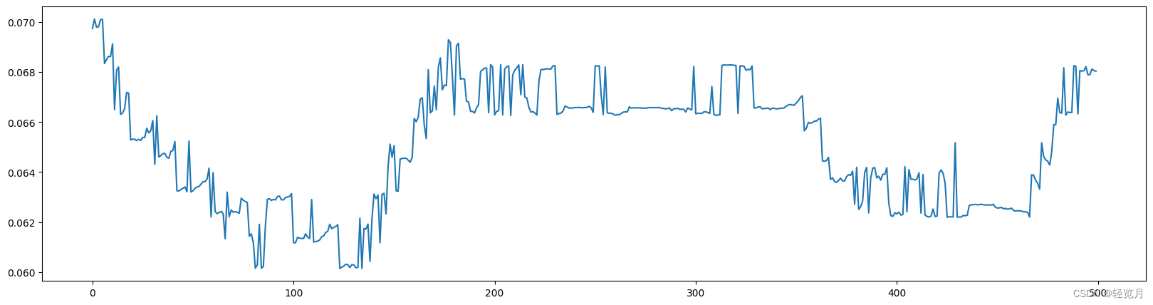
<Figure size 2000x500 with 1 Axes>

3.2.3 特征工程

在特征工程阶段，构建基本的时间特征，提取小时、分钟等相关特征，主要是为了刻画不同时间阶段可能存在的差异性信息。需要注意数据是分多个文件存储的，所以需要进行文件合并，然后在进行后续的工作。

# 时间相关特征
train_df['hour'] = train_df['time'].apply(lambda x:int(x.split(':')[0]))
test_df['hour'] = test_df['time'].apply(lambda x:int(x.split(':')[0]))

train_df['minute'] = train_df['time'].apply(lambda x:int(x.split(':')[1]))
test_df['minute'] = test_df['time'].apply(lambda x:int(x.split(':')[1]))

# 入模特征
cols = [f for f in test_df.columns if f not in ['uuid','time','file']]

3.2.4 模型训练与验证

选择使用CatBoost模型，也是通常作为机器学习比赛的基线模型，在不需要过程调参的情况下也能得到比较稳定的分数。这里使用五折交叉验证的方式进行数据切分验证，最终将五个模型结果取平均作为最终提交。

def cv_model(clf, train_x, train_y, test_x, clf_name, seed = 2023):
    folds = 5
    kf = KFold(n_splits=folds, shuffle=True, random_state=seed)
    oof = np.zeros([train_x.shape[0], 3])
    test_predict = np.zeros([test_x.shape[0], 3])
    cv_scores = []
    
    for i, (train_index, valid_index) in enumerate(kf.split(train_x, train_y)):
        print('************************************ {} ************************************'.format(str(i+1)))
        trn_x, trn_y, val_x, val_y = train_x.iloc[train_index], train_y[train_index], train_x.iloc[valid_index], train_y[valid_index]
       
        if clf_name == "cat":
            params = {'learning_rate': 0.2, 'depth': 6, 'bootstrap_type':'Bernoulli','random_seed':2023,
                      'od_type': 'Iter', 'od_wait': 100, 'random_seed': 11, 'allow_writing_files': False,
                      'loss_function': 'MultiClass'}
            
            model = clf(iterations=100, **params)
            model.fit(trn_x, trn_y, eval_set=(val_x, val_y),
                      metric_period=20,
                      use_best_model=True, 
                      cat_features=[],
                      verbose=1)
            
            val_pred  = model.predict_proba(val_x)
            test_pred = model.predict_proba(test_x)
        
        oof[valid_index] = val_pred
        test_predict += test_pred / kf.n_splits
        
        F1_score = f1_score(val_y, np.argmax(val_pred, axis=1), average='macro')
        cv_scores.append(F1_score)
        print(cv_scores)
        
    return oof, test_predict
    
for label in ['label_5','label_10','label_20','label_40','label_60']:
    print(f'=================== {label} ===================')
    cat_oof, cat_test = cv_model(CatBoostClassifier, train_df[cols], train_df[label], test_df[cols], 'cat')
    train_df[label] = np.argmax(cat_oof, axis=1)
    test_df[label] = np.argmax(cat_test, axis=1)

本次比赛采用macro-F1 score进行评价，取label_5, label_10, label_20, label_40, label_60五项中的最高分作为最终得分，所以在初次建模的时候对应五个目标都需要进行建模，确定分数最高的目标，之后进行优化的时候仅需对最优目标进行建模即可，大大节省时间，聚焦单个目标优化。

3.2.5 结果输出

提交结果需要符合提交样例结果，然后将文件夹进行压缩成zip格式提交。

test_df.head(5)

   uuid  date      time  sym   n_close  amount_delta  n_midprice    n_bid1  \
0     0    65  13:10:03    0 -0.027661     1334257.0   -0.027048 -0.027486   
1     1    65  13:10:06    0 -0.026611      194481.0   -0.026961 -0.027311   
2     2    65  13:10:09    0 -0.026611      122263.0   -0.026786 -0.026961   
3     3    65  13:10:12    0 -0.026786      216809.0   -0.025910 -0.026786   
4     4    65  13:10:15    0 -0.026611       44481.0   -0.025648 -0.026261   

       n_bsize1    n_bid2  ...   n_ask5  n_asize5  \
0  1.250056e-05 -0.027661  ... -0.02416  0.000008   
1  5.984310e-07 -0.027486  ... -0.02416  0.000008   
2  9.641389e-07 -0.027136  ... -0.02451  0.000002   
3  1.496078e-07 -0.026961  ... -0.02416  0.000008   
4  2.161001e-07 -0.026611  ... -0.02416  0.000008   

                          file  hour  minute  label_5  label_10  label_20  \
0  snapshot_sym0_date65_pm.csv    13      10        1         1         1   
1  snapshot_sym0_date65_pm.csv    13      10        1         1         1   
2  snapshot_sym0_date65_pm.csv    13      10        1         1         1   
3  snapshot_sym0_date65_pm.csv    13      10        1         1         1   
4  snapshot_sym0_date65_pm.csv    13      10        1         1         1   

   label_40  label_60  
0         1         1  
1         1         1  
2         1         1  
3         1         1  
4         1         1  

[5 rows x 35 columns]

import pandas as pd
import os


# 指定输出文件夹路径
output_dir = './submit'

# 如果文件夹不存在则创建
if not os.path.exists(output_dir):
    os.makedirs(output_dir)

# 首先按照'file'字段对 dataframe 进行分组
grouped = test_df.groupby('file')

# 对于每一个group进行处理
for file_name, group in grouped:
    # 选择你所需要的列
    selected_cols = group[['uuid', 'label_5', 'label_10', 'label_20', 'label_40', 'label_60']]
    
    # 将其保存为csv文件，file_name作为文件名
    selected_cols.to_csv(os.path.join(output_dir, f'{file_name}'), index=False)

# 现在就可以得到答案的压缩包啦~~~
_ = !zip -r submit.zip submit/

4. 进阶实战

在baseline阶段，我们使用CatBoost完成了解决机器学习问题的全部流程，得到了基础的分数。在进阶实践部分，将在原有Baseline基础上做更多优化，一般优化思路，从特征工程与模型中来思考。

优化方法建议：

1. 提取更多特征：在数据挖掘比赛中，特征总是最终制胜法宝，去思考什么信息可以帮助我们提高预测精准度，然后将其转化为特征输入到模型。对于本次赛题可以从业务角度构建特征，在量化交易方向中，常说的因子与机器学习中的特征基本一致，趋势因子、收益波动率因子、买卖压力、同成交量衰减、斜率 价差/深度，可以围绕成交量、买价和卖价进行构建。也可以从时间序列预测角度构建特征，比如历史平移特征、差分特征、和窗口统计特征。

2. 尝试不同的模型：模型间存在很大的差异，预测结果也会不一样，比赛的过程就是不断的实验和试错的过程，通过不断的实验寻找最佳模型，同时帮助自身加强模型的理解能力。

4.1 特征选择

这里主要构建了当前时间特征、历史平移特征、差分特征、和窗口统计特征；每种特征都是有理可据的，具体说明如下：

（1）当前时间特征：围绕买卖价格和买卖量进行构建，暂时只构建买一卖一和买二卖二相关特征，进行优化时可以加上其余买卖信息；

（2）历史平移特征：通过历史平移获取上个阶段的信息；

（3）差分特征：可以帮助获取相邻阶段的增长差异，描述数据的涨减变化情况。在此基础上还可以构建相邻数据比值变化、二阶差分等；

（4）窗口统计特征：窗口统计可以构建不同的窗口大小，然后基于窗口范围进统计均值、最大值、最小值、中位数、方差的信息，可以反映最近阶段数据的变化情况。

# 特征代码一览（无需运行这里）

# 为了保证时间顺序的一致性，故进行排序
train_df = train_df.sort_values(['file','time'])
test_df = test_df.sort_values(['file','time'])

# 当前时间特征
# 围绕买卖价格和买卖量进行构建
# 暂时只构建买一卖一和买二卖二相关特征，进行优化时可以加上其余买卖信息
train_df['wap1'] = (train_df['n_bid1']*train_df['n_bsize1'] + train_df['n_ask1']*train_df['n_asize1'])/(train_df['n_bsize1'] + train_df['n_asize1'])
test_df['wap1'] = (test_df['n_bid1']*test_df['n_bsize1'] + test_df['n_ask1']*test_df['n_asize1'])/(test_df['n_bsize1'] + test_df['n_asize1'])

train_df['wap2'] = (train_df['n_bid2']*train_df['n_bsize2'] + train_df['n_ask2']*train_df['n_asize2'])/(train_df['n_bsize2'] + train_df['n_asize2'])
test_df['wap2'] = (test_df['n_bid2']*test_df['n_bsize2'] + test_df['n_ask2']*test_df['n_asize2'])/(test_df['n_bsize2'] + test_df['n_asize2'])

train_df['wap_balance'] = abs(train_df['wap1'] - train_df['wap2'])
train_df['price_spread'] = (train_df['n_ask1'] - train_df['n_bid1']) / ((train_df['n_ask1'] + train_df['n_bid1'])/2)
train_df['bid_spread'] = train_df['n_bid1'] - train_df['n_bid2']
train_df['ask_spread'] = train_df['n_ask1'] - train_df['n_ask2']
train_df['total_volume'] = (train_df['n_asize1'] + train_df['n_asize2']) + (train_df['n_bsize1'] + train_df['n_bsize2'])
train_df['volume_imbalance'] = abs((train_df['n_asize1'] + train_df['n_asize2']) - (train_df['n_bsize1'] + train_df['n_bsize2']))

test_df['wap_balance'] = abs(test_df['wap1'] - test_df['wap2'])
test_df['price_spread'] = (test_df['n_ask1'] - test_df['n_bid1']) / ((test_df['n_ask1'] + test_df['n_bid1'])/2)
test_df['bid_spread'] = test_df['n_bid1'] - test_df['n_bid2']
test_df['ask_spread'] = test_df['n_ask1'] - test_df['n_ask2']
test_df['total_volume'] = (test_df['n_asize1'] + test_df['n_asize2']) + (test_df['n_bsize1'] + test_df['n_bsize2'])
test_df['volume_imbalance'] = abs((test_df['n_asize1'] + test_df['n_asize2']) - (test_df['n_bsize1'] + test_df['n_bsize2']))

# 历史平移
# 获取历史信息
for val in ['wap1','wap2','wap_balance','price_spread','bid_spread','ask_spread','total_volume','volume_imbalance']:
    for loc in [1,5,10,20,40,60]:
        train_df[f'file_{val}_shift{loc}'] = train_df.groupby(['file'])[val].shift(loc)
        test_df[f'file_{val}_shift{loc}'] = test_df.groupby(['file'])[val].shift(loc)
    
# 差分特征
# 获取与历史数据的增长关系
for val in ['wap1','wap2','wap_balance','price_spread','bid_spread','ask_spread','total_volume','volume_imbalance']:
    for loc in [1,5,10,20,40,60]:
        train_df[f'file_{val}_diff{loc}'] = train_df.groupby(['file'])[val].diff(loc)
        test_df[f'file_{val}_diff{loc}'] = test_df.groupby(['file'])[val].diff(loc)
    
# 窗口统计
# 获取历史信息分布变化信息
# 可以尝试更多窗口大小已经统计方式，如min、max、median等
for val in ['wap1','wap2','wap_balance','price_spread','bid_spread','ask_spread','total_volume','volume_imbalance']:
    train_df[f'file_{val}_win7_mean'] = train_df.groupby(['file'])[val].transform(lambda x: x.rolling(window=7, min_periods=3).mean())
    train_df[f'file_{val}_win7_std'] = train_df.groupby(['file'])[val].transform(lambda x: x.rolling(window=7, min_periods=3).std())
    
    test_df[f'file_{val}_win7_mean'] = test_df.groupby(['file'])[val].transform(lambda x: x.rolling(window=7, min_periods=3).mean())
    test_df[f'file_{val}_win7_std'] = test_df.groupby(['file'])[val].transform(lambda x: x.rolling(window=7, min_periods=3).std())

4.2 模型融合

模型融合代码参考：

定义cv_model函数，内部可以选择使用lightgbm、xgboost和catboost模型，可以依次跑完这三个模型，然后将三个模型的结果进行取平均进行融合。

# 无需运行这里

def cv_model(clf, train_x, train_y, test_x, clf_name, seed = 2023):
    folds = 5
    kf = KFold(n_splits=folds, shuffle=True, random_state=seed)
    oof = np.zeros([train_x.shape[0], 3])
    test_predict = np.zeros([test_x.shape[0], 3])
    cv_scores = []
    
    for i, (train_index, valid_index) in enumerate(kf.split(train_x, train_y)):
        print('************************************ {} ************************************'.format(str(i+1)))
        trn_x, trn_y, val_x, val_y = train_x.iloc[train_index], train_y[train_index], train_x.iloc[valid_index], train_y[valid_index]
        
        if clf_name == "lgb":
            train_matrix = clf.Dataset(trn_x, label=trn_y)
            valid_matrix = clf.Dataset(val_x, label=val_y)
            params = {
                'boosting_type': 'gbdt',
                'objective': 'multiclass',
                'num_class':3,
                'min_child_weight': 6,
                'num_leaves': 2 ** 6,
                'lambda_l2': 10,
                'feature_fraction': 0.8,
                'bagging_fraction': 0.8,
                'bagging_freq': 4,
                'learning_rate': 0.35,
                'seed': 2023,
                'nthread' : 16,
                'verbose' : -1,
            }
            model = clf.train(params, train_matrix, 2000, valid_sets=[train_matrix, valid_matrix],
                              categorical_feature=[], verbose_eval=1000, early_stopping_rounds=100)
            val_pred = model.predict(val_x, num_iteration=model.best_iteration)
            test_pred = model.predict(test_x, num_iteration=model.best_iteration)
        
        if clf_name == "xgb":
            xgb_params = {
              'booster': 'gbtree', 
              'objective': 'multi:softprob',
              'num_class':3,
              'max_depth': 5,
              'lambda': 10,
              'subsample': 0.7,
              'colsample_bytree': 0.7,
              'colsample_bylevel': 0.7,
              'eta': 0.35,
              'tree_method': 'hist',
              'seed': 520,
              'nthread': 16
              }
            train_matrix = clf.DMatrix(trn_x , label=trn_y)
            valid_matrix = clf.DMatrix(val_x , label=val_y)
            test_matrix = clf.DMatrix(test_x)
            
            watchlist = [(train_matrix, 'train'),(valid_matrix, 'eval')]
            
            model = clf.train(xgb_params, train_matrix, num_boost_round=2000, evals=watchlist, verbose_eval=1000, early_stopping_rounds=100)
            val_pred  = model.predict(valid_matrix)
            test_pred = model.predict(test_matrix)
            
        if clf_name == "cat":
            params = {'learning_rate': 0.35, 'depth': 5, 'bootstrap_type':'Bernoulli','random_seed':2023,
                      'od_type': 'Iter', 'od_wait': 100, 'random_seed': 11, 'allow_writing_files': False,
                      'loss_function': 'MultiClass'}
            
            model = clf(iterations=2000, **params)
            model.fit(trn_x, trn_y, eval_set=(val_x, val_y),
                      metric_period=1000,
                      use_best_model=True, 
                      cat_features=[],
                      verbose=1)
            
            val_pred  = model.predict_proba(val_x)
            test_pred = model.predict_proba(test_x)
        
        oof[valid_index] = val_pred
        test_predict += test_pred / kf.n_splits
        
        F1_score = f1_score(val_y, np.argmax(val_pred, axis=1), average='macro')
        cv_scores.append(F1_score)
        print(cv_scores)
        
    return oof, test_predict

# 参考demo,具体对照baseline实践部分调用cv_model函数
# 选择lightgbm模型
lgb_oof, lgb_test = cv_model(lgb, train_df[cols], train_df['label_5'], test_df[cols], 'lgb')
# 选择xgboost模型
xgb_oof, xgb_test = cv_model(xgb, train_df[cols], train_df['label_5'], test_df[cols], 'xgb')
# 选择catboost模型
cat_oof, cat_test = cv_model(CatBoostClassifier, train_df[cols], train_df['label_5'], test_df[cols], 'cat')

# 进行取平均融合
final_test = (lgb_test + xgb_test + cat_test) / 3

将结果取平均进行融合是比较基础的融合的方式，另外一种经典融合方式为stacking，stacking是一种分层模型集成框架。以两层为例，第一层由多个基学习器组成，其输入为原始训练集，第二层的模型则是以第一层基学习器的输出作为特征加入训练集进行再训练，从而得到完整的stacking模型。

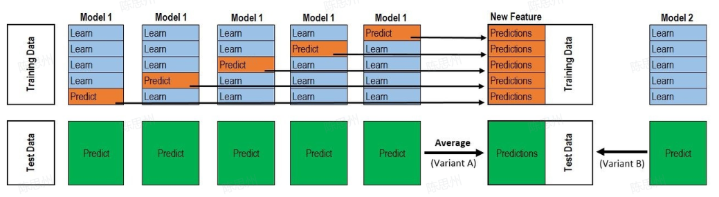
第一层：（类比cv_model函数）

1. 划分训练数据为K折（5折为例，每次选择其中四份作为训练集，一份作为验证集）；

2. 针对各个模型RF、ET、GBDT、XGB，分别进行5次训练，每次训练保留一份样本用作训练时的验证，训练完成后分别对Validation set，Test set进行预测，对于Test set一个模型会对应5个预测结果，将这5个结果取平均；对于Validation set一个模型经过5次交叉验证后，所有验证集数据都含有一个标签。此步骤结束后：**5个验证集（总数相当于训练集全部）在每个模型下分别有一个预测标签，每行数据共有4个标签（4个算法模型），测试集每行数据也拥有四个标签（4个模型分别预测得到的） **

第二层：（类比stack_model函数）

1. 将训练集中的四个标签外加真实标签当作五列新的特征作为新的训练集，选取一个训练模型，根据新的训练集进行训练，然后应用测试集的四个标签组成的测试集进行预测作为最终的result。

Stacking参考代码：

需要特别注意，代码给出的是解决二分类问题的流程，对于多分类问题大家可以自行尝试。

def stack_model(oof_1, oof_2, oof_3, predictions_1, predictions_2, predictions_3, y):
    '''
    输入的oof_1, oof_2, oof_3可以对应lgb_oof，xgb_oof，cat_oof
    predictions_1, predictions_2, predictions_3对应lgb_test，xgb_test，cat_test
    '''
    train_stack = pd.concat([oof_1, oof_2, oof_3], axis=1)
    test_stack = pd.concat([predictions_1, predictions_2, predictions_3], axis=1)
    
    oof = np.zeros((train_stack.shape[0],))
    predictions = np.zeros((test_stack.shape[0],))
    scores = []
    
    from sklearn.model_selection import RepeatedKFold
    folds = RepeatedKFold(n_splits=5, n_repeats=2, random_state=2021)
    
    for fold_, (trn_idx, val_idx) in enumerate(folds.split(train_stack, train_stack)): 
        print("fold n°{}".format(fold_+1))
        trn_data, trn_y = train_stack.loc[trn_idx], y[trn_idx]
        val_data, val_y = train_stack.loc[val_idx], y[val_idx]
        
        clf = Ridge(random_state=2021)
        clf.fit(trn_data, trn_y)

        oof[val_idx] = clf.predict(val_data)
        predictions += clf.predict(test_stack) / (5 * 2)
        
        score_single = roc_auc_score(val_y, oof[val_idx])
        scores.append(score_single)
        print(f'{fold_+1}/{5}', score_single)
    print('mean: ',np.mean(scores))
   
    return oof, predictions

4.3 优化后的Baseline一键运行~~

# 可一键运行~

_ = !unzip -qo data/data233139/AI量化模型预测挑战赛公开数据.zip
_ = !pip install --upgrade catboost xgboost lightgbm

import os
import shutil
import numpy as np
import pandas as pd
from catboost import CatBoostClassifier
from sklearn.model_selection import StratifiedKFold, KFold, GroupKFold
from sklearn.metrics import accuracy_score, f1_score, roc_auc_score, log_loss, mean_squared_log_error
import xgboost as xgb
import lightgbm as lgb
import tqdm, sys, os, gc, argparse, warnings
warnings.filterwarnings('ignore')
import paddle

if paddle.device.is_compiled_with_cuda():
    device = "GPU"
else:
    device = "CPU"


# 定义要检测的路径
path_to_check = 'AI量化模型预测挑战赛公开数据/test/'

# 检测.ipynb_checkpoints是否存在于这个路径中
for foldername in os.listdir(path_to_check):
    if foldername == '.ipynb_checkpoints':
        # 构造完整的文件夹路径
        full_path = os.path.join(path_to_check, foldername)
        
        # 删除文件夹及其所有内容
        shutil.rmtree(full_path)
        print(f'Removed .ipynb_checkpoints directory at: {full_path}')

# 读取数据
path = 'AI量化模型预测挑战赛公开数据/'

train_files = os.listdir(path+'train')
train_df = pd.DataFrame()
for filename in tqdm.tqdm(train_files):
    tmp = pd.read_csv(path+'train/'+filename)
    tmp['file'] = filename
    train_df = pd.concat([train_df, tmp], axis=0, ignore_index=True)

test_files = os.listdir(path+'test')
test_df = pd.DataFrame()
for filename in tqdm.tqdm(test_files):
    tmp = pd.read_csv(path+'test/'+filename)
    tmp['file'] = filename
    test_df = pd.concat([test_df, tmp], axis=0, ignore_index=True)


# 时间相关特征
train_df['hour'] = train_df['time'].apply(lambda x:int(x.split(':')[0]))
test_df['hour'] = test_df['time'].apply(lambda x:int(x.split(':')[0]))

train_df['minute'] = train_df['time'].apply(lambda x:int(x.split(':')[1]))
test_df['minute'] = test_df['time'].apply(lambda x:int(x.split(':')[1]))


# 为了保证时间顺序的一致性，故进行排序
train_df = train_df.sort_values(['file','time'])
test_df = test_df.sort_values(['file','time'])

# 当前时间特征
# 围绕买卖价格和买卖量进行构建
# 暂时只构建买一卖一和买二卖二相关特征，进行优化时可以加上其余买卖信息
train_df['wap1'] = (train_df['n_bid1']*train_df['n_bsize1'] + train_df['n_ask1']*train_df['n_asize1'])/(train_df['n_bsize1'] + train_df['n_asize1'])
test_df['wap1'] = (test_df['n_bid1']*test_df['n_bsize1'] + test_df['n_ask1']*test_df['n_asize1'])/(test_df['n_bsize1'] + test_df['n_asize1'])

train_df['wap2'] = (train_df['n_bid2']*train_df['n_bsize2'] + train_df['n_ask2']*train_df['n_asize2'])/(train_df['n_bsize2'] + train_df['n_asize2'])
test_df['wap2'] = (test_df['n_bid2']*test_df['n_bsize2'] + test_df['n_ask2']*test_df['n_asize2'])/(test_df['n_bsize2'] + test_df['n_asize2'])

train_df['wap_balance'] = abs(train_df['wap1'] - train_df['wap2'])
train_df['price_spread'] = (train_df['n_ask1'] - train_df['n_bid1']) / ((train_df['n_ask1'] + train_df['n_bid1'])/2)
train_df['bid_spread'] = train_df['n_bid1'] - train_df['n_bid2']
train_df['ask_spread'] = train_df['n_ask1'] - train_df['n_ask2']
train_df['total_volume'] = (train_df['n_asize1'] + train_df['n_asize2']) + (train_df['n_bsize1'] + train_df['n_bsize2'])
train_df['volume_imbalance'] = abs((train_df['n_asize1'] + train_df['n_asize2']) - (train_df['n_bsize1'] + train_df['n_bsize2']))

test_df['wap_balance'] = abs(test_df['wap1'] - test_df['wap2'])
test_df['price_spread'] = (test_df['n_ask1'] - test_df['n_bid1']) / ((test_df['n_ask1'] + test_df['n_bid1'])/2)
test_df['bid_spread'] = test_df['n_bid1'] - test_df['n_bid2']
test_df['ask_spread'] = test_df['n_ask1'] - test_df['n_ask2']
test_df['total_volume'] = (test_df['n_asize1'] + test_df['n_asize2']) + (test_df['n_bsize1'] + test_df['n_bsize2'])
test_df['volume_imbalance'] = abs((test_df['n_asize1'] + test_df['n_asize2']) - (test_df['n_bsize1'] + test_df['n_bsize2']))

# 历史平移
# 获取历史信息
for val in ['wap1','wap2','wap_balance','price_spread','bid_spread','ask_spread','total_volume','volume_imbalance']:
    for loc in [1,5,10,20,40,60]:
        train_df[f'file_{val}_shift{loc}'] = train_df.groupby(['file'])[val].shift(loc)
        test_df[f'file_{val}_shift{loc}'] = test_df.groupby(['file'])[val].shift(loc)
    
# 差分特征
# 获取与历史数据的增长关系
for val in ['wap1','wap2','wap_balance','price_spread','bid_spread','ask_spread','total_volume','volume_imbalance']:
    for loc in [1,5,10,20,40,60]:
        train_df[f'file_{val}_diff{loc}'] = train_df.groupby(['file'])[val].diff(loc)
        test_df[f'file_{val}_diff{loc}'] = test_df.groupby(['file'])[val].diff(loc)
    
# 窗口统计
# 获取历史信息分布变化信息
# 可以尝试更多窗口大小已经统计方式，如min、max、median等
for val in ['wap1','wap2','wap_balance','price_spread','bid_spread','ask_spread','total_volume','volume_imbalance']:
    train_df[f'file_{val}_win7_mean'] = train_df.groupby(['file'])[val].transform(lambda x: x.rolling(window=7, min_periods=3).mean())
    train_df[f'file_{val}_win7_std'] = train_df.groupby(['file'])[val].transform(lambda x: x.rolling(window=7, min_periods=3).std())
    
    test_df[f'file_{val}_win7_mean'] = test_df.groupby(['file'])[val].transform(lambda x: x.rolling(window=7, min_periods=3).mean())
    test_df[f'file_{val}_win7_std'] = test_df.groupby(['file'])[val].transform(lambda x: x.rolling(window=7, min_periods=3).std())

def cv_model(clf, train_x, train_y, test_x, clf_name, seed = 2023):
    folds = 5
    kf = KFold(n_splits=folds, shuffle=True, random_state=seed)
    oof = np.zeros([train_x.shape[0], 3])
    test_predict = np.zeros([test_x.shape[0], 3])
    cv_scores = []
    
    for i, (train_index, valid_index) in enumerate(kf.split(train_x, train_y)):
        print('************************************ {} ************************************'.format(str(i+1)))
        trn_x, trn_y, val_x, val_y = train_x.iloc[train_index], train_y[train_index], train_x.iloc[valid_index], train_y[valid_index]
        
        if clf_name == "lgb":
            train_matrix = clf.Dataset(trn_x, label=trn_y)
            valid_matrix = clf.Dataset(val_x, label=val_y)
            params = {
                'boosting_type': 'gbdt',
                'objective': 'multiclass',
                'num_class':3,
                'min_child_weight': 6,
                'num_leaves': 2 ** 6,
                'lambda_l2': 10,
                'feature_fraction': 0.8,
                'bagging_fraction': 0.8,
                'bagging_freq': 4,
                'learning_rate': 0.1,
                'seed': 2023,
                'nthread' : 16,
                'verbose' : -1,
            }
            model = clf.train(params, train_matrix, 200, valid_sets=[train_matrix, valid_matrix],
                              categorical_feature=[])
            val_pred = model.predict(val_x, num_iteration=model.best_iteration)
            test_pred = model.predict(test_x, num_iteration=model.best_iteration)
        
        if clf_name == "xgb":
            xgb_params = {
              'booster': 'gbtree', 
              'objective': 'multi:softprob',
              'num_class':3,
              'max_depth': 5,
              'lambda': 10,
              'subsample': 0.7,
              'colsample_bytree': 0.7,
              'colsample_bylevel': 0.7,
              'eta': 0.1,
              'tree_method': 'hist',
              'seed': 520,
              'nthread': 16,
              'tree_method': 'gpu_hist',
              }
            train_matrix = clf.DMatrix(trn_x , label=trn_y)
            valid_matrix = clf.DMatrix(val_x , label=val_y)
            test_matrix = clf.DMatrix(test_x)
            
            watchlist = [(train_matrix, 'train'),(valid_matrix, 'eval')]
            
            model = clf.train(xgb_params, train_matrix, num_boost_round=200, evals=watchlist)
            val_pred  = model.predict(valid_matrix)
            test_pred = model.predict(test_matrix)
            
        if clf_name == "cat":
            params = {'learning_rate': 0.1, 'depth': 5, 'bootstrap_type':'Bernoulli','random_seed':2023,
                      'od_type': 'Iter', 'od_wait': 100, 'random_seed': 11, 'allow_writing_files': False,
                      'loss_function': 'MultiClass', "task_type": device}
            
            model = clf(iterations=200, **params)
            model.fit(trn_x, trn_y, eval_set=(val_x, val_y),
                      metric_period=50,
                      use_best_model=True, 
                      cat_features=[],
                      verbose=1)
            
            val_pred  = model.predict_proba(val_x)
            test_pred = model.predict_proba(test_x)
        
        oof[valid_index] = val_pred
        test_predict += test_pred / kf.n_splits
        
        F1_score = f1_score(val_y, np.argmax(val_pred, axis=1), average='macro')
        cv_scores.append(F1_score)
        print(cv_scores)
        
    return oof, test_predict
    
# 处理train_x和test_x中的NaN值
train_df = train_df.fillna(0)
test_df = test_df.fillna(0)

# 处理train_x和test_x中的Inf值
train_df = train_df.replace([np.inf, -np.inf], 0)
test_df = test_df.replace([np.inf, -np.inf], 0)

# 入模特征
cols = [f for f in test_df.columns if f not in ['uuid','time','file']]
for label in ['label_5','label_10','label_20','label_40','label_60']:
    print(f'=================== {label} ===================')
    # 选择lightgbm模型
    lgb_oof, lgb_test = cv_model(lgb, train_df[cols], train_df[label], test_df[cols], 'lgb')
    # 选择xgboost模型
    xgb_oof, xgb_test = cv_model(xgb, train_df[cols], train_df[label], test_df[cols], 'xgb')
    # 选择catboost模型
    cat_oof, cat_test = cv_model(CatBoostClassifier, train_df[cols], train_df[label], test_df[cols], 'cat')

    # 进行取平均融合
    final_test = (lgb_test + xgb_test + cat_test) / 3

    test_df[label] = np.argmax(final_test, axis=1)


import pandas as pd
import os

# 检查并删除'submit'文件夹
if os.path.exists('./submit'):
    shutil.rmtree('./submit')
    print("Removed the 'submit' directory.")

# 检查并删除'submit.zip'文件
if os.path.isfile('./submit.zip'):
    os.remove('./submit.zip')
    print("Removed the 'submit.zip' file.")

# 指定输出文件夹路径
output_dir = './submit'

# 如果文件夹不存在则创建
if not os.path.exists(output_dir):
    os.makedirs(output_dir)

# 首先按照'file'字段对 dataframe 进行分组
grouped = test_df.groupby('file')

# 对于每一个group进行处理
for file_name, group in grouped:
    # 选择你所需要的列
    selected_cols = group[['uuid', 'label_5', 'label_10', 'label_20', 'label_40', 'label_60']]
    
    # 将其保存为csv文件，file_name作为文件名
    selected_cols.to_csv(os.path.join(output_dir, f'{file_name}'), index=False)


_ = !zip -r submit.zip submit/

到这里大家可能会有疑惑，为何没有优化后的代码比优化后的还高，这是因为，特征数量增多以后，训练所需要的时间很明显应该更多才对，然而在这里为了大家运行的速度考虑，仅设置了iterations=100，这通常来说是不够的，想要取得更好的成绩可以考虑将其设置的更高，