KA-001 26 Kaggle Solutions: C2 House Price Prediction（Regularized Liner Model）

Solutions for C2 House Price Prediction（Regularized Liner Model）

---

1 Introduction

1.1 Competition Description

 Ask a home buyer to describe their dream house, and they probably won’t begin with the height of the basement ceiling or the proximity to an east-west railroad. But this playground competition’s dataset proves that much more influences price negotiations than the number of bedrooms or a white-picket fence.

 With 79 explanatory variables describing (almost) every aspect of residential homes in Ames, Iowa, this competition challenges you to predict the final price of each home

1.2 Statement

Originator：Alexandru Papiu
Analyzed：Tinky Wu

1.3 Basic Ideas

2 Data Processing

2.1 Import package and load data

import pandas as pd
import numpy as np
import seaborn as sns
import matplotlib
import matplotlib.pyplot as plt
from scipy.stats import skew
from scipy.stats.stats import pearsonr
%matplotlib inline

train = pd.read_csv("../input/train.csv")
test = pd.read_csv("../input/test.csv")

2.2 Data exploration

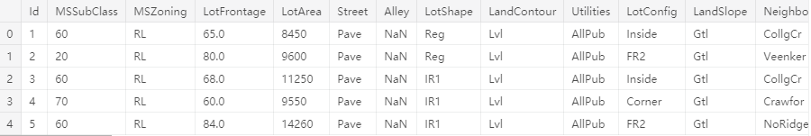
First, let’s look at the basic data

train.head()

data.info()

2.3 Preprocessing

all_data = pd.concat((train.loc[:,'MSSubClass':'SaleCondition'],
					  test.loc[:,'MSSubClass':'SaleCondition'])) 
					  #Process the dataset together

matplotlib.rcParams['figure.figsize'] = (12.0, 6.0)
#{ rcParams } Set the Image pixel, 'rc' means configuration

prices = pd.DataFrame({"price":train["SalePrice"], 
					   "log(price + 1)":np.log1p(train["SalePrice"])})
prices.hist()

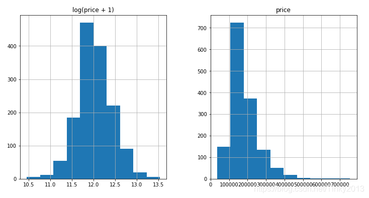
We can see that we have transformed srewed values after the log transform

train["SalePrice"] = np.log1p(train["SalePrice"]) 
#log transform the target

numeric_feats = all_data.dtypes[all_data.dtypes != "object"].index
#log transform skewed numeric features
#If all the data in the column is not object, the column will be selected

skewed_feats = train[numeric_feats].apply(lambda x: skew(x.dropna())) #compute skewness, just for the training set

skewed_feats = skewed_feats[skewed_feats > 0.75]
#Choose the numeric column that skewness>0.75

skewed_feats = skewed_feats.index
all_data[skewed_feats] = np.log1p(all_data[skewed_feats])
#Transform the chosen columns

2.4 One-Hot Encoding

#fill the missing value and create matrices for sklearn
all_data = pd.get_dummies(all_data)
all_data = all_data.fillna(all_data.mean()) #filling NA's with the mean of the column
X_train = all_data[:train.shape[0]]
X_test = all_data[train.shape[0]:]
y = train.SalePrice

3 Modeling

After the simple transform, now using regularized linear regression models
The author tried both l_1(Lasso) and l_2(Ridge) regularization
He also defined a function that returns the cross-validation rmse to evaluate the model

3.1 Basic Model: Ridge & Lasso

from sklearn.linear_model import Ridge, RidgeCV, ElasticNet, LassoCV, LassoLarsCV
from sklearn.model_selection import cross_val_score

【rmse】：root-mean-square error: Measures the deviation between Observed value and Truth-value

def rmse_cv(model):
    rmse= np.sqrt(-cross_val_score(model, X_train, y, scoring="neg_mean_squared_error", cv = 5))
    return(rmse)
model_ridge = Ridge()

higher alpha means more restriction on coefficient ‘w’ (May improve the generalization performance and avoid overfit)

alphas = [0.05, 0.1, 0.3, 1, 3, 5, 10, 15, 30, 50, 75]  # Adjusting parameters
cv_ridge = [rmse_cv(Ridge(alpha = alpha)).mean() for alpha in alphas]
#Visualization: alphas-rmse
cv_ridge = pd.Series(cv_ridge, index = alphas)
cv_ridge.plot(title = "Validation - Just Do It")
plt.xlabel("alpha")
plt.ylabel("rmse")

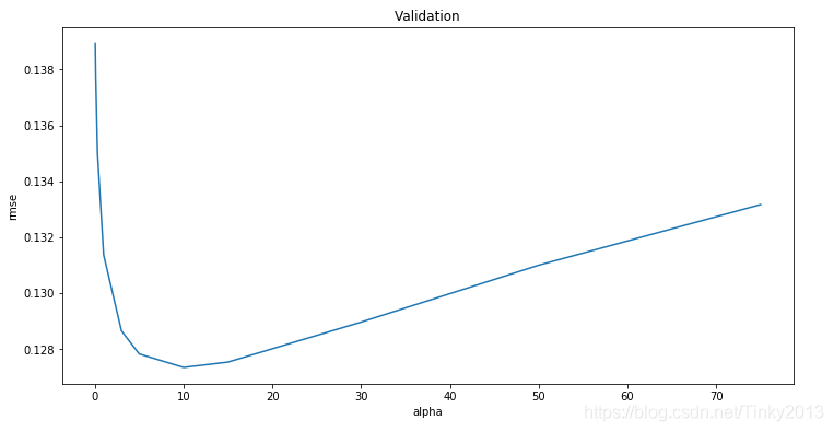
Now we check the Root Mean Squared Logarithmic Error(The smaller the better)

cv_ridge.min()

Next we try Lasso

model_lasso = LassoCV(alphas = [1, 0.1, 0.001, 0.0005]).fit(X_train, y)
rmse_cv(model_lasso).mean()

Lasso does feature selection for you - setting coefficients of features it deems unimportant to zero. It performs somewhat better than ridge model.

3.2 Check the model

Check how many features it choose

coef = pd.Series(model_lasso.coef_, index = X_train.columns)
print("Lasso picked " + str(sum(coef != 0)) + " variables and eliminated the other " +  str(sum(coef == 0)) + " variables")

Take a look directly at what the most important coefficients are

imp_coef = pd.concat([coef.sort_values().head(10),coef.sort_values().tail(10)])
matplotlib.rcParams['figure.figsize'] = (8.0, 10.0)
imp_coef.plot(kind = "barh")
plt.title("Coefficients in the Lasso Model")

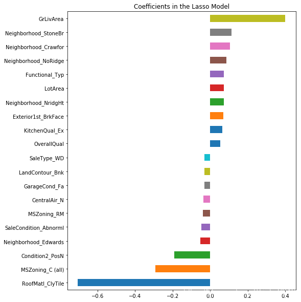
These are actual coefficients ’w‘ in your model
It’s easier to explain the predicted price concluded by the model

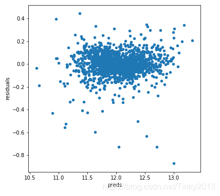
Now we check the residuals

matplotlib.rcParams['figure.figsize'] = (6.0, 6.0)
preds = pd.DataFrame({"preds":model_lasso.predict(X_train), "true":y})
preds["residuals"] = preds["true"] - preds["preds"]
preds.plot(x = "preds", y = "residuals",kind = "scatter")

3.3 Add another model: xgboost

import xgboost as xgb
dtrain = xgb.DMatrix(X_train, label = y)
dtest = xgb.DMatrix(X_test)
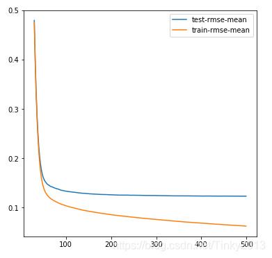
params = {"max_depth":2, "eta":0.1}
model = xgb.cv(params, dtrain,  num_boost_round=500, early_stopping_rounds=100)
model.loc[30:,["test-rmse-mean", "train-rmse-mean"]].plot()#visualize the rmse-mean changing

model_xgb = xgb.XGBRegressor(n_estimators=360, max_depth=2, learning_rate=0.1) #the params were tuned using xgb.cv
model_xgb.fit(X_train, y)

4 Predicting

xgb_preds = np.expm1(model_xgb.predict(X_test))
lasso_preds = np.expm1(model_lasso.predict(X_test))
predictions = pd.DataFrame({"xgb":xgb_preds, "lasso":lasso_preds})
predictions.plot(x = "xgb", y = "lasso", kind = "scatter")

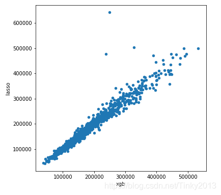
Take a weighted average

preds = 0.75*lasso_preds + 0.25*xgb_preds #Take a weighted average of uncorrelated results
solution = pd.DataFrame({"id":test.Id, "SalePrice":preds})
solution.to_csv("ridge_sol.csv", index = False)

5 Results

If there’s any flow, please point out. Thank you!