深度学习目标检测里用到的各种loss积累
1. binary_cross_entropy
Binary cross entropy常用与二分类问题,比如two-stage目标检测函数在第一个阶段RPN提出proposals的时候,需要对其进行正负样本的分类,针对分类的损失就是Binary cross entropy。其公式如下:
Loss = − 1 N ∑ i = 1 N y i ⋅ log ( p ( y i ) ) + ( 1 − y i ) ⋅ log ( 1 − p ( y i ) ) \text { Loss }=-\frac{1}{\mathrm{~N}} \sum_{\mathrm{i}=1}^{\mathrm{N}} \mathrm{y}_{\mathrm{i}} \cdot \log \left(\mathrm{p}\left(\mathrm{y}_{\mathrm{i}}\right)\right)+\left(1-\mathrm{y}_{\mathrm{i}}\right) \cdot \log \left(1-\mathrm{p}\left(\mathrm{y}_{\mathrm{i}}\right)\right) Loss =− N1i=1∑Nyi⋅log(p(yi))+(1−yi)⋅log(1−p(yi))
公式很好理解,具体理论参考:快速理解binary cross entropy 二元交叉熵
def binary_cross_entropy(pred,  #我们预测的为正样本的分数
                         label, #真实的标签
                         weight=None,
                         reduction='mean',
                         avg_factor=None,
                         class_weight=None,
                         ignore_index=-100,
                         avg_non_ignore=False):

    # The default value of ignore_index is the same as F.cross_entropy
    ignore_index = -100 if ignore_index is None else ignore_index

    if pred.dim() != label.dim():  #这里判断是否为二进制损失
        label, weight, valid_mask = _expand_onehot_labels(   #将label的维度扩展成与pred一样
            label, weight, pred.size(-1), ignore_index)
    else:
        # should mask out the ignored elements
        valid_mask = ((label >= 0) & (label != ignore_index)).float()
        if weight is not None:
            # The inplace writing method will have a mismatched broadcast
            # shape error if the weight and valid_mask dimensions
            # are inconsistent such as (B,N,1) and (B,N,C).
            weight = weight * valid_mask
        else:
            weight = valid_mask

    # average loss over non-ignored elements
    if (avg_factor is None) and avg_non_ignore and reduction == 'mean':
        avg_factor = valid_mask.sum().item()

    # weighted element-wise losses
    weight = weight.float()
    loss = F.binary_cross_entropy_with_logits(
        pred, label.float(), pos_weight=class_weight, reduction='none')
    # do the reduction for the weighted loss
    loss = weight_reduce_loss(
        loss, weight, reduction=reduction, avg_factor=avg_factor)

    return loss

#二进制交叉熵损失特有的函数
def _expand_onehot_labels(labels, label_weights, label_channels, ignore_index):
    """Expand onehot labels to match the size of prediction."""
    bin_labels = labels.new_full((labels.size(0), label_channels), 0)    #[196608, 1]
    valid_mask = (labels >= 0) & (labels != ignore_index)                #[196608]都是true
    inds = torch.nonzero(                   #非0元素的索引,即不仅为正样本,并且有效的元素的索引
        valid_mask & (labels < label_channels), as_tuple=False)

    if inds.numel() > 0:
        bin_labels[inds, labels[inds]] = 1                               #正样本为1,其余为0

    valid_mask = valid_mask.view(-1, 1).expand(labels.size(0),           #[196608, 1]都是true
                                               label_channels).float()
    if label_weights is None:
        bin_label_weights = valid_mask
    else:
        bin_label_weights = label_weights.view(-1, 1).repeat(1, label_channels) #正负样本都为1,其余为0
        bin_label_weights *= valid_mask

    return bin_labels, bin_label_weights, valid_mask
这里用的是F.binary_cross_entropy_with_logits函数,该函数会自动添加sigmoid运算,即将Sigmoid层和BCELoss合并在一个类中。在数值上比使用一个简单的Sigmoid和一个BCELoss更稳定,通过将操作合并到一个层中,利用log-sum-exp技巧来实现数值稳定性。
参数reduction的作用:
ℓ ( x , y ) = { mean ( L ) , if reduction = ‘mean’; sum ( L ) , if reduction = ‘sum’ \ell(x, y)=\left\{\begin{array}{ll} \operatorname{mean}(L), & \text { if reduction }=\text { ‘mean'; } \\ \operatorname{sum}(L), & \text { if reduction }= \text { ‘sum' } \end{array}\right. ℓ(x,y)={
mean(L),sum(L), if reduction = ‘mean’; if reduction = ‘sum’
2. smooth_l1_loss
对于边框预测回归问题,通常也可以选择平方损失函数(L2损失),但L2范数的缺点是当存在离群点(outliers)的时候,这些点会占loss的主要组成部分。比如说真实值为1,预测10次,有一次预测值为1000,其余次的预测值为1左右,显然loss值主要由1000主宰。所以FastRCNN采用稍微缓和一点绝对损失函数(smooth L1损失),它是随着误差线性增长,而不是平方增长。
注意:smooth L1和L1-loss函数的区别在于,L1-loss在0点处导数不唯一,可能影响收敛。smooth L1的解决办法是在0点附近使用平方函数使得它更加平滑。
- L2 loss:
L 2 = ∣ f ( x ) − Y ∣ 2 L 2 ′ = 2 f ′ ( x ) ( f ( x ) − Y ) \begin{array}{l} L_{2}=|f(x)-Y|^{2} \\ L_{2}^{\prime}=2 f^{\prime}(x)(f(x)-Y) \end{array} L2=∣f(x)−Y∣2L2′=2f′(x)(f(x)−Y) - L1 loss:
L 1 = ∣ f ( x ) − Y ∣ L 1 ′ = ± f ′ ( x ) \begin{array}{l} L_{1}=|f(x)-Y| \\ L_{1}^{\prime}= \pm f^{\prime}(x) \end{array} L1=∣f(x)−Y∣L1′=±f′(x) - Smooth L1 loss
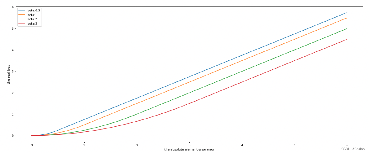
l n = { 0.5 ( x n − y n ) 2 / beta, if ∣ x n − y n ∣ < beta ∣ x n − y n ∣ − 0.5 ∗ beta, otherwise l_{n}=\left\{\begin{array}{ll} 0.5\left(x_{n}-y_{n}\right)^{2} / \text { beta, } & \text { if }\left|x_{n}-y_{n}\right|<\text { beta } \\ \left|x_{n}-y_{n}\right|-0.5 * \text { beta, } & \text { otherwise } \end{array}\right. ln={ 0.5(xn−yn)2/ beta, ∣xn−yn∣−0.5∗ beta, if ∣xn−yn∣< beta otherwise
loss曲线:
def smooth_l1_loss(pred, target, beta=1.0):
    """Smooth L1 loss.

    Args:
        pred (torch.Tensor): The prediction.
        target (torch.Tensor): The learning target of the prediction.
        beta (float, optional): The threshold in the piecewise function.
            Defaults to 1.0.

    Returns:
        torch.Tensor: Calculated loss
    """
    assert beta > 0
    if target.numel() == 0:
        return pred.sum() * 0

    assert pred.size() == target.size()
    diff = torch.abs(pred - target)
    loss = torch.where(diff < beta, 0.5 * diff * diff / beta,
                       diff - 0.5 * beta)
    return loss