(一)KITTI数据集用于3D目标检测

KITTI数据集介绍

数据基本情况

KITTI是德国卡尔斯鲁厄科技学院和丰田芝加哥研究院开源的数据集,最早发布于2012年03月20号。

对应的论文Are we ready for Autonomous Driving? The KITTI Vision Benchmark Suite发表在CVPR2012上。

KITTI数据集搜集自德国卡尔斯鲁厄市，包括市区/郊区/高速公路等交通场景。采集于2011年09月26/28/29/30号及10月03号的白天。

KITTI数据采集使用的平台如下图，

上面平台中包括

• 2个140万像素的黑白相机
• 2个140万像素的彩色相机
• 4个爱特蒙特光学镜头
• 1个64线 Velodyne 3D激光扫描仪
• 1个OXTS RT3003 惯导系统

从上图中可以看到

• 相机的坐标系，Z轴是朝前的，Y轴是朝下的，整个坐标系是右手坐标系。
• 激光雷达的X轴是朝向正前方，Z轴是竖直向上的，Y轴根据右手定则确定
• IMU/GPS系统的坐标系朝向和激光雷达一致

总结，KITTI数据集是由4个相机，1个激光雷达，1个IMU/GPS惯导系统共同组成，我们所要厘清的是这6个传感器之间的坐标系关系和时间同步信息。

关于传感器的尺寸参数可以参考下图，

在[date]-drive-sync-[sqquence]目录下存放了6个传感器对应的采集数据文件夹。

- image00
- image01
- image02
- image03
- oxts
- velodyne-points

• 时间戳，在velodyne-points文件夹下有三个时间戳文件

  • timestamps_start.txt，激光扫描仪一周开始扫描的时间
  • timestamps_end.txt，激光扫描仪一周扫描结束的时间
  • timestamps.txt 激光扫描到正前方触发相机拍照的时间。

• 图像数据

  • 图像是裁剪掉了引擎盖和天空之后的图像
  • 图像是去畸变之后的数据

• OSTX数据，每一帧存储了包括经纬度/速度/加速度等30个不同的字段值

• 雷达数据

  • 浮点数的二进制文件，每个点由4个浮点数组成，雷达坐标系下的x,y,z坐标，激光的反射强度r
  • 每扫描一次，大约得到了120000个3D点。
  • 激光雷达绕垂直轴逆时针转动

传感器标定及时间同步

整个系统以激光雷达旋转一周为1帧，激光雷达旋转到某个特定位置的时候，通过一个弹簧片的物理接触触发相机拍照，IMU无法通过这种触发的方式采集数据，但IMU数据采集的频率达到了100HZ，对IMU采集的数据记录时间戳，选择与相机采集时间最接近的作为当前帧的数据，最大时间误差为5ms。

相机标定，相机内外参标定使用的方法是A toolbox for
automatic calibration of range and camera sensors using a single shot,所有的相机中心都已对齐，即他们都在相同的XY平面上，这便于图像的校正(去除天空和引擎盖)

每天开始采集数据前，都会对整个数据采集系统进行标定，以免传感器间位置的偏移。

在每天的date_calib.zip文件夹下，有3个文本文件，

• calib_cam_to_cam.txt
  
  其中最后三个参数值的解释下，$s_{rect}^{(i)}$表示的是校正后(去除多余的天空和引擎盖)图像的大小；${\mathbf{R}}_{rect}^{(i)}$是校正所用的旋转矩阵；${\mathbf{P}}_{rect}^{(i)}$是校正所用投影矩阵。 i ∈ { 0 , 1 , 2 , 3 } i\in\{0,1,2,3\} i∈{ 0,1,2,3}表示相机的序号，0表示左侧灰度相机，1表示右侧灰度相机，2表示左侧彩色相机，3表示右侧彩色相机。左侧灰度相机0作为参考相机坐标系，参考相机坐标系下的一个3D点$\mathbf{x}=(x,y,z,1)$,要变换到第i个相机图像中，可使用如下关系：$\mathbf{y}={\mathbf{P}}_{rect}^{(i)}{\mathbf{R}}_{rect}^{(0)}\mathbf{x}$

• calib_velo_to_cam.txt，KITTI数据集激光雷达也是相对于左侧灰度相机0标定的，由激光到相机的旋转矩阵${\mathbf{R}}_{velo}^{cam}$和平移向量${\mathbf{t}}_{velo}^{cam}$组成，齐次变换矩阵可以写成，
  $${\mathbf{T}}_{velo}^{cam}=\left(\begin{array}{cc}{R}_{velo}^{cam}& t_{velo}^{cam}\\ 0& 1\end{array}\right)$$
  如此，将雷达坐标系下的3D点变换到第$i$个相机坐标系下时的公式为:$$\mathbf{y}={\mathbf{P}}_{rect}^{(i)}{\mathbf{R}}_{rect}^{(0)}{\mathbf{T}}_{velo}^{cam}\mathbf{x}$$

• calib_imu_to_velo.txt,这个文件中保存有imu坐标系到激光坐标系下的齐次变换矩阵${\mathbf{T}}_{imu}^{velo}$,如此，将IMU坐标系下的一个3D点变换到第i个图像中的像素坐标的公式可写为
  $$\mathbf{y}={\mathbf{P}}_{rect}^{(i)}{\mathbf{R}}_{rect}^{(0)}{\mathbf{T}}_{velo}^{cam}{\mathbf{T}}_{imu}^{velo}\mathbf{x}$$

用于3D目标检测

最初数据集支持的任务有双目，光流和里程计。后来，陆陆续续支持了深度估计、2D目标检测、3D目标检测、BEV目标检测、语义分割、实例分割、多目标追踪等任务。

在目标检测中，定义的类别有8种：

Car/Van/Truck/Pedestrian/Person_sitting/Cyclist/Tram/Misc(其他)。

对3D对象的标注是在激光雷达坐标系下进行的，不过值得注意的一点是现在3D目标检测只由检测框中心点坐标xyz,检测框的长宽高length/width/height和检测框的偏航角yaw这7个自由度组成。

不过这里也有个很容易引起歧义的问题length/width/height分别是对应xyz的哪个轴呢？从下图可以看出length对应dx，width对应dy,height对应dz。整个3D框的标注在激光雷达坐标系下。

KITTI 3D目标检测数据集包括7481张训练数据，7518张测试数据。尽管KITTI数据集中包含了标注了8种对象，只有Car/Pedestrian标注的比较充分，KITTI官方用来评估算法, KITTI BenchMark中使用的3D检测框类别有3个，分别是Car/Pedestrian/Cyclist。

下载的3D目标检测数据集包含的文件夹有

• image_02， 左目彩色png格式的图像
• label_02, 左目彩色图像中标注的对象标签
• calib, 传感器之间的坐标转换关系
• velodyne, 激光点云数据
• plane,在激光坐标系下，路面的平面方程

标签文件中每一行内容如下：

Pedestrian 0.00 0 -0.20 712.40 143.00 810.73 307.92 1.89 0.48 1.20 1.84 1.47 8.41 0.01

包含的字段有，

• type 目标的类型，如Car/Van…，1个字段
• truncated 浮点数0-1，目标对象离开相机视野的比例，1个字段
• occluded 整数0,1,2,3，0:全部可见，1:部分遮挡，2:大部分未遮挡，3:未知，1个字段
• alpha，对象的观测角，1个字段$[-\pi ,\pi ]$
• bbox，2D检测框像素坐标，x1,y1,x2,y2，4个字段
• dimensions,3D对象的尺寸，height,width,length,单位是米,3个字段
• location，3D对象在相机坐标系下的中心坐标xyz，单位是m
• rotation_y，yaw角，偏航角,$[-\pi ,\pi ]$
• score, 目标对象的评分，用来计算ROC曲线或MAP。

相机坐标系中的点可以通过calib中的变换矩阵变换到图像像素坐标中。

rotation_y和alpha的区别在于，alpha度量的是相机中心到对象中心的角度。rotation_y度量的是对象绕相机坐标系y轴的转角yaw。以汽车为例，当一辆车在相机坐标系下位于x轴方向时，其rotation_y角为零，无论这辆车在x,z平面的哪个位置。而对于alpha角来说，仅当汽车在相机坐标系下z轴上时，alpha角为零，偏离z轴时，alpha角都不为零。

将激光点云投影到左目彩色图像中可以使用的公式为：X=P2*R0_rect*Tr_vel_to_cam*Y。

R0_rect是3x3的校正矩阵，Tr_vel_to_cam是3x4的雷达变换到相机坐标系下的变换矩阵。

代码实战

使用open3d读取点云

import numpy as np
import struct
import open3d as o3d

def convert_kitti_bin_to_pcd(binFilePath):
    size_float = 4
    list_pcd = []
    with open(binFilePath, "rb") as f:
        byte = f.read(size_float * 4)
        print(byte)
        while byte:
            x, y, z, intensity = struct.unpack("ffff", byte)
            list_pcd.append([x, y, z])
            byte = f.read(size_float * 4)
    np_pcd = np.asarray(list_pcd)
    pcd = o3d.geometry.PointCloud()
    pcd.points = o3d.utility.Vector3dVector(np_pcd)
    return pcd

bs = "/xx/xx/data/code/mmdetection3d/demo/data/kitti/000008.bin"
pcds = convert_kitti_bin_to_pcd(bs)
o3d.visualization.draw_geometries([pcds])

# save
o3d.io.write_point_cloud('000008.pcd', pcds, write_ascii=False, compressed=False, print_progress=False)

通过numpy读取，

def load_bin(bin_file):
    data = np.fromfile(bin_file, np.float32).reshape((-1, 4))
    data = data[:, :-1]
    pcd = o3d.geometry.PointCloud()
    pcd.points = o3d.utility.Vector3dVector(data)
    return pcd

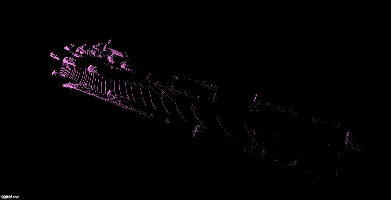
上面的代码可以读取并可视化点云数据，且保存成pcd格式的点云。

选取的3D目标检测任务数据集training/image_02/000008.png，

对应的标签文件000008.txt,

Car 0.88 3 -0.69 0.00 192.37 402.31 374.00 1.60 1.57 3.23 -2.70 1.74 3.68 -1.29
Car 0.00 1 2.04 334.85 178.94 624.50 372.04 1.57 1.50 3.68 -1.17 1.65 7.86 1.90
Car 0.34 3 -1.84 937.29 197.39 1241.00 374.00 1.39 1.44 3.08 3.81 1.64 6.15 -1.31
Car 0.00 1 -1.33 597.59 176.18 720.90 261.14 1.47 1.60 3.66 1.07 1.55 14.44 -1.25
Car 0.00 0 1.74 741.18 168.83 792.25 208.43 1.70 1.63 4.08 7.24 1.55 33.20 1.95
Car 0.00 0 -1.65 884.52 178.31 956.41 240.18 1.59 1.59 2.47 8.48 1.75 19.96 -1.25

将其画在000008.png上为，

import cv2
img = cv2.imread(img_s)
with open(label_s) as f:
    lines = f.read().split("\n")[:-1]
for item in lines:
    boxes = item.split()[4:8]
    boxes = [float(x) for x in boxes]
    bb = np.array(boxes, dtype=np.int32)
    cv2.rectangle(img, bb[:2], bb[-2:], (0,0,255), 1)
cv2.imwrite("/xx/xx/data/code/mmdetection3d/demo/data/kitti/08_res.png", img)

看左下角两个检测框，边缘部分标注的并不好。

对应的点云数据为：

KITTI3D目标检测的数据标签给出的3D中心点的坐标是在左目彩色相机坐标系中。

使用Open3D可视化检测框的代码可以参考，

"""
from https://github.com/dtczhl/dtc-KITTI-For-
Beginners.git
"""
import matplotlib.pyplot as plt
import matplotlib.image as mping
import numpy as np
import os
import open3d as o3d
import open3d.visualization as o3d_vis
from shapely.geometry import Point
from shapely.geometry.polygon import Polygon


MARKER_COLOR = {
    
    
    'Car': [1, 0, 0],               # red
    'DontCare': [0, 0, 0],          # black
    'Pedestrian': [0, 0, 1],        # blue
    'Van': [1, 1, 0],               # yellow
    'Cyclist': [1, 0, 1],           # magenta
    'Truck': [0, 1, 1],             # cyan
    'Misc': [0.5, 0, 0],            # maroon
    'Tram': [0, 0.5, 0],            # green
    'Person_sitting': [0, 0, 0.5]}  # navy

# image border width
BOX_BORDER_WIDTH = 5

# point size
POINT_SIZE = 0.005


def show_object_in_image(img_filename, label_filename):
    img = mping.imread(img_filename)
    with open(label_filename) as f_label:
        lines = f_label.readlines()
        for line in lines:
            line = line.strip('\n').split()
            left_pixel, top_pixel, right_pixel, bottom_pixel = [int(float(line[i])) for i in range(4, 8)]
            box_border_color = MARKER_COLOR[line[0]]
            for i in range(BOX_BORDER_WIDTH):
                img[top_pixel+i, left_pixel:right_pixel, :] = box_border_color
                img[bottom_pixel-i, left_pixel:right_pixel, :] = box_border_color
                img[top_pixel:bottom_pixel, left_pixel+i, :] = box_border_color
                img[top_pixel:bottom_pixel, right_pixel-i, :] = box_border_color
    plt.imshow(img)
    plt.show()

def show_object_in_point_cloud(point_cloud_filename, label_filename, calib_filename):
    pc_data = np.fromfile(point_cloud_filename, '<f4')  # little-endian float32
    pc_data = np.reshape(pc_data, (-1, 4))
    cloud = o3d.geometry.PointCloud()
    cloud.points = o3d.utility.Vector3dVector(pc_data[:,:-1])
    pc_color = np.ones((len(pc_data), 3))
    calib = load_kitti_calib(calib_filename)
    rot_axis = 2
    with open(label_filename) as f_label:
        lines = f_label.readlines()
        bboxes_3d = []
        for line in lines:
            line = line.strip('\n').split()
            point_color = MARKER_COLOR[line[0]]
            veloc, dims, rz, box3d_corner = camera_coordinate_to_point_cloud(line[8:15], calib['Tr_velo_to_cam'])
            bboxes_3d.append(np.concatenate((veloc, dims, np.array([rz]))))
        bboxes_3d = np.array(bboxes_3d)
        print(bboxes_3d.shape)
        lines = []
        for i in range(len(bboxes_3d)):
            center = bboxes_3d[i, 0:3]
            dim = bboxes_3d[i, 3:6]
            yaw = np.zeros(3)
            yaw[rot_axis] = bboxes_3d[i, 6]
            rot_mat = o3d.geometry.get_rotation_matrix_from_xyz(yaw)
            # bottom center to gravity center
            center[rot_axis] += dim[rot_axis] / 2

            box3d = o3d.geometry.OrientedBoundingBox(center, rot_mat, dim)
            
            line_set = o3d.geometry.LineSet.create_from_oriented_bounding_box(
                box3d)
            line_set.paint_uniform_color(np.array(point_color) / 255.)
            lines.append(line_set)
        
        for i, v in enumerate(pc_data):
            if point_in_cube(v[:3], box3d_corner) is True:
                pc_color[i, :] = point_color
                
        cloud.colors = o3d.utility.Vector3dVector(pc_color)
        o3d_vis.draw([*lines, cloud])

def point_in_cube(point, cube):
    z_min = np.amin(cube[:, 2], 0)
    z_max = np.amax(cube[:, 2], 0)

    if point[2] > z_max or point[2] < z_min:
        return False

    point = Point(point[:2])
    polygon = Polygon(cube[:4, :2])

    return polygon.contains(point)


def load_kitti_calib(calib_file):
    """
    This script is copied from https://github.com/AI-liu/Complex-YOLO
    """
    with open(calib_file) as f_calib:
        lines = f_calib.readlines()

    P0 = np.array(lines[0].strip('\n').split()[1:], dtype=np.float32)
    P1 = np.array(lines[1].strip('\n').split()[1:], dtype=np.float32)
    P2 = np.array(lines[2].strip('\n').split()[1:], dtype=np.float32)
    P3 = np.array(lines[3].strip('\n').split()[1:], dtype=np.float32)
    R0_rect = np.array(lines[4].strip('\n').split()[1:], dtype=np.float32)
    Tr_velo_to_cam = np.array(lines[5].strip('\n').split()[1:], dtype=np.float32)
    Tr_imu_to_velo = np.array(lines[6].strip('\n').split()[1:], dtype=np.float32)

    return {
    
    'P0': P0, 'P1': P1, 'P2': P2, 'P3': P3, 'R0_rect': R0_rect,
            'Tr_velo_to_cam': Tr_velo_to_cam.reshape(3, 4),
            'Tr_imu_to_velo': Tr_imu_to_velo}


def camera_coordinate_to_point_cloud(box3d, Tr):
    """
    This script is copied from https://github.com/AI-liu/Complex-YOLO
    """
    def project_cam2velo(cam, Tr):
        T = np.zeros([4, 4], dtype=np.float32)
        T[:3, :] = Tr
        T[3, 3] = 1
        T_inv = np.linalg.inv(T)
        lidar_loc_ = np.dot(T_inv, cam)
        lidar_loc = lidar_loc_[:3]
        return lidar_loc.reshape(1, 3)

    def ry_to_rz(ry):
        angle = -ry - np.pi / 2

        if angle >= np.pi:
            angle -= np.pi
        if angle < -np.pi:
            angle = 2 * np.pi + angle
        return angle

    h, w, l, tx, ty, tz, ry = [float(i) for i in box3d]
    cam = np.ones([4, 1])
    cam[0] = tx
    cam[1] = ty
    cam[2] = tz
    t_lidar = project_cam2velo(cam, Tr)

    Box = np.array([[-l / 2, -l / 2, l / 2, l / 2, -l / 2, -l / 2, l / 2, l / 2],
                    [w / 2, -w / 2, -w / 2, w / 2, w / 2, -w / 2, -w / 2, w / 2],
                    [0, 0, 0, 0, h, h, h, h]])

    rz = ry_to_rz(ry)

    rotMat = np.array([
        [np.cos(rz), -np.sin(rz), 0.0],
        [np.sin(rz), np.cos(rz), 0.0],
        [0.0, 0.0, 1.0]])

    velo_box = np.dot(rotMat, Box)

    cornerPosInVelo = velo_box + np.tile(t_lidar, (8, 1)).T

    box3d_corner = cornerPosInVelo.transpose()
    dims = np.array([l, w, h])
    # t_lidar: the x, y coordinator of the center of the object
    # box3d_corner: the 8 corners
    print(t_lidar.shape)
    return t_lidar.reshape(-1), dims, rz, box3d_corner.astype(np.float32)


if __name__ == '__main__':

    # updates
    ROOT = "/media/lx/data/code/mmdetection3d/demo/data/kitti"
    IMG_DIR = f'{
      
      ROOT}/image_2'
    LABEL_DIR = f'{
      
      ROOT}/label_2'
    POINT_CLOUD_DIR = f'{
      
      ROOT}/velo'
    CALIB_DIR = f'{
      
      ROOT}/calib'

    # id for viewing
    file_id = 8

    img_filename = os.path.join(IMG_DIR, '{0:06d}.png'.format(file_id))
    label_filename = os.path.join(LABEL_DIR, '{0:06d}.txt'.format(file_id))
    pc_filename = os.path.join(POINT_CLOUD_DIR, '{0:06d}.bin'.format(file_id))
    calib_filename = os.path.join(CALIB_DIR, '{0:06d}.txt'.format(file_id))

    # show object in image
    show_object_in_image(img_filename, label_filename)

    # show object in point cloud
    show_object_in_point_cloud(pc_filename, label_filename, calib_filename)

可视化的结果为:

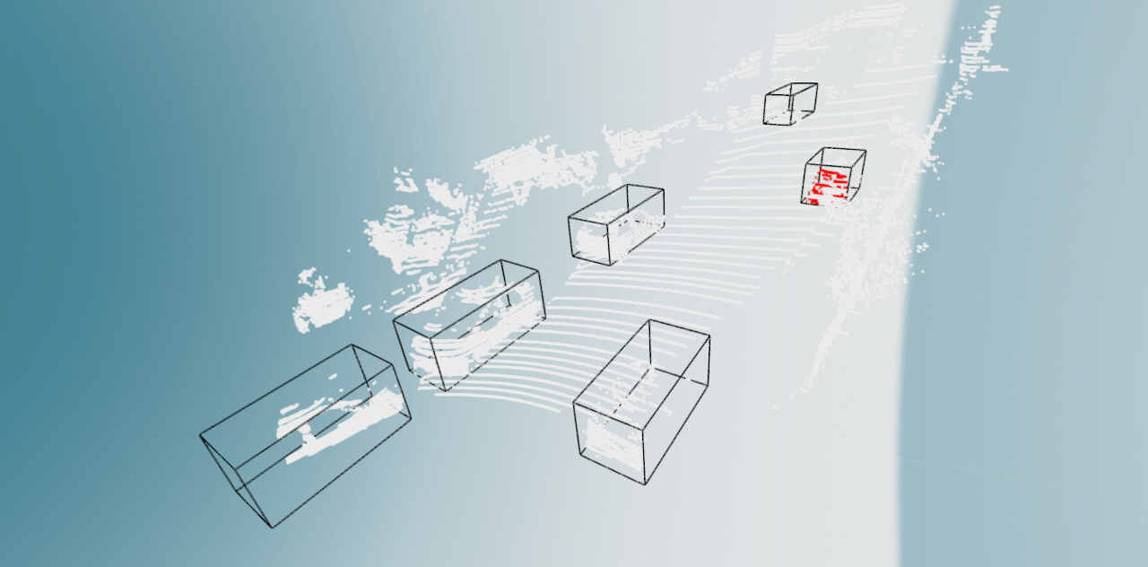
以上，就可以对KITTI数据集用于3D目标检测任务的情况有一个基本的认识了，后面用到多模态的时候再补充如何结合2D检测框一起来做目标的识别和定位。

• 1.https://www.cvlibs.net/datasets/kitti/eval_object.php?obj_benchmark=3d
• 2.https://github.com/dtczhl/dtc-KITTI-For-
  Beginners.git