MobileNet v1网络
MobileNet网络专注于移动端或者嵌入式设备中的轻量级CNN网络。相比传统卷积神经网络,在准确率小幅降低的前提下大大减少模型参数与运算量。相比于VGG16准确率减少了0.9%,但模型参数只有VGG的1/32.
1.Depthwise Convolution(大大减少运算量和参数数量)
2.增加了超参数α和β。
MobileNet v2网络
相比于MovileNet v1网络,准确率更高,模型更小。
1.Inverted Residuals(倒残差结构)
2.Linear Bottlenecks
MovileNet v3网络
1.更新了Block(bneck,加入SE模块,更新了激活函数 )
2.使用NAS搜索参数(Neural Architecture Search)
3.重新设计耗时层结构
ShuffleNet v1网络
1.提出了channel shuffle的思想
2.ShuffleNet Unit中全是GConv和DWConv
阅读论文《HybridSN: Exploring 3-D–2-DCNN Feature Hierarchy for Hyperspectral Image Classification》,思考3D卷积和2D卷积的区别。
把代码敲入 Colab 运行,网络部分需要自己完成。
#Spectral Python (SPy)是一个用于处理高光谱图像数据的纯Python模块。
#它具有读取、显示、操作和分类高光谱图像的功能。之所以用它是因为这个对多波段图像的支持更好
! pip install spectral
#导入所使用的库
import numpy as np
import matplotlib.pyplot as plt
import scipy.io as sio
from sklearn.decomposition import PCA
from sklearn.model_selection import train_test_split
from sklearn.metrics import confusion_matrix, accuracy_score, classification_report, cohen_kappa_score
import spectral
import torch
import torchvision
import torch.nn as nn
import torch.nn.functional as F
import torch.optim as optim
#导入云盘中上传的文件
from google.colab import drive
drive.mount('/content/drive/')
import scipy.io as sio
import os
filepath = os.path.join('/content/drive/My Drive/Deeplearning/Indian_pines_corrected.mat')
filepath1 = os.path.join('/content/drive/My Drive/Deeplearning/Indian_pines_gt.mat')
#定义HybridSN类
class_num = 16
class HybridSN(nn.Module):
  def __init__(self,num_classes=16):
    super(HybridSN,self).__init__()
    self.conv1 = nn.Conv3d(1,8,(7,3,3))
    self.bn1=nn.BatchNorm3d(8)

    self.conv2 = nn.Conv3d(8,16,(5,3,3))
    self.bn2=nn.BatchNorm3d(16)

    self.conv3 = nn.Conv3d(16,32,(3,3,3))
    self.bn3=nn.BatchNorm3d(32)

    self.conv4 = nn.Conv2d(576,64,(3,3))
    self.bn4=nn.BatchNorm2d(64)

    self.drop = nn.Dropout(p=0.4)

    self.fc1 = nn.Linear(18496,256)
    self.fc2 = nn.Linear(256,128)
    self.fc3 = nn.Linear(128,num_classes)

    self.relu = nn.ReLU()

    self.softmax = nn.Softmax(dim=1)

  def forward(self,x):
    out = self.relu(self.bn1(self.conv1(x)))
    out = self.relu(self.bn2(self.conv2(out)))
    out = self.relu(self.bn3(self.conv3(out)))

    out = out.view(-1,out.shape[1]*out.shape[2],out.shape[3],out.shape[4])
    out = self.relu(self.bn4(self.conv4(out)))

    out = out.view(out.size(0),-1)
    out = self.fc1(out)
    out = self.drop(out)
    out = self.relu(out)
    out = self.fc2(out)
    out = self.drop(out)
    out = self.relu(out)
    out = self.fc3(out)
    # out = self.softmax(out)
    return out


# 随机输入,测试网络结构是否通
x = torch.randn(1,1,30,25,25)
net = HybridSN()
y = net(x)
print(y.shape)
# 创建数据集
# 对高光谱数据 X 应用 PCA 变换
def applyPCA(X, numComponents):
    newX = np.reshape(X, (-1, X.shape[2]))
    pca = PCA(n_components=numComponents, whiten=True)
    newX = pca.fit_transform(newX)
    newX = np.reshape(newX, (X.shape[0], X.shape[1], numComponents))
    return newX

# 对单个像素周围提取 patch 时,边缘像素就无法取了,因此,给这部分像素进行 padding 操作
def padWithZeros(X, margin=2):
    newX = np.zeros((X.shape[0] + 2 * margin, X.shape[1] + 2* margin, X.shape[2]))
    x_offset = margin
    y_offset = margin
    newX[x_offset:X.shape[0] + x_offset, y_offset:X.shape[1] + y_offset, :] = X
    return newX

# 在每个像素周围提取 patch ,然后创建成符合 keras 处理的格式
def createImageCubes(X, y, windowSize=5, removeZeroLabels = True):
    # 给 X 做 padding
    margin = int((windowSize - 1) / 2)
    zeroPaddedX = padWithZeros(X, margin=margin)
    # split patches
    patchesData = np.zeros((X.shape[0] * X.shape[1], windowSize, windowSize, X.shape[2]))
    patchesLabels = np.zeros((X.shape[0] * X.shape[1]))
    patchIndex = 0
    for r in range(margin, zeroPaddedX.shape[0] - margin):
        for c in range(margin, zeroPaddedX.shape[1] - margin):
            patch = zeroPaddedX[r - margin:r + margin + 1, c - margin:c + margin + 1]
            patchesData[patchIndex, :, :, :] = patch
            patchesLabels[patchIndex] = y[r-margin, c-margin]
            patchIndex = patchIndex + 1
    if removeZeroLabels:
        patchesData = patchesData[patchesLabels>0,:,:,:]
        patchesLabels = patchesLabels[patchesLabels>0]
        patchesLabels -= 1
    return patchesData, patchesLabels

def splitTrainTestSet(X, y, testRatio, randomState=345):
    X_train, X_test, y_train, y_test = train_test_split(X, y, test_size=testRatio, random_state=randomState, stratify=y)
    return X_train, X_test, y_train, y_test
#读取并创建数据集
# 地物类别
class_num = 16
X = sio.loadmat(filepath)['indian_pines_corrected']
y = sio.loadmat(filepath1)['indian_pines_gt']
# 用于测试样本的比例
test_ratio = 0.90
# 每个像素周围提取 patch 的尺寸
patch_size = 25
# 使用 PCA 降维,得到主成分的数量
pca_components = 30
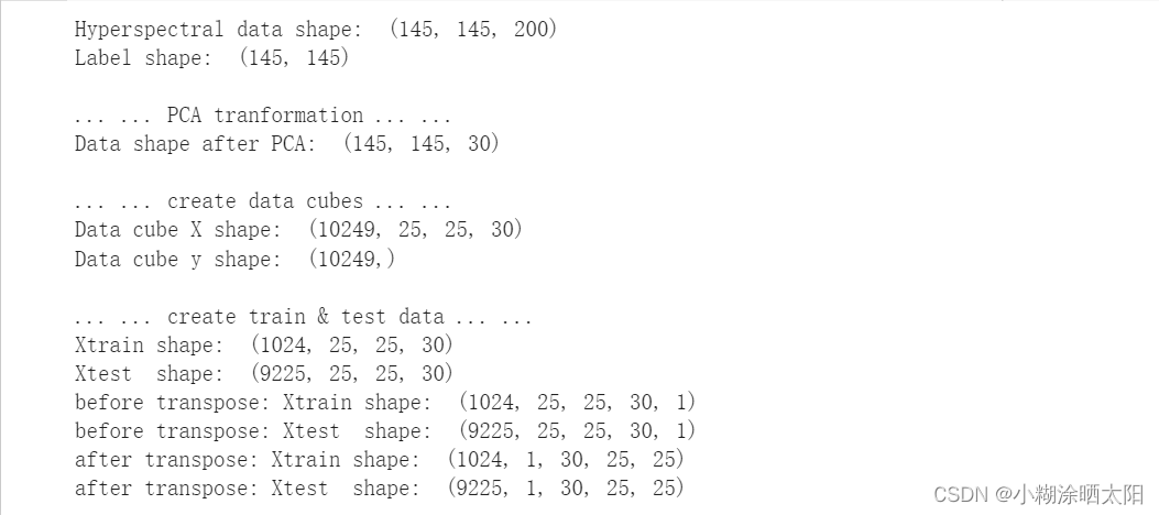
print('Hyperspectral data shape: ', X.shape)
print('Label shape: ', y.shape)
print('\n... ... PCA tranformation ... ...')
X_pca = applyPCA(X, numComponents=pca_components)
print('Data shape after PCA: ', X_pca.shape)
print('\n... ... create data cubes ... ...')
X_pca, y = createImageCubes(X_pca, y, windowSize=patch_size)
print('Data cube X shape: ', X_pca.shape)
print('Data cube y shape: ', y.shape)
print('\n... ... create train & test data ... ...')
Xtrain, Xtest, ytrain, ytest = splitTrainTestSet(X_pca, y, test_ratio)
print('Xtrain shape: ', Xtrain.shape)
print('Xtest shape: ', Xtest.shape)
# 改变 Xtrain, Ytrain 的形状,以符合 keras 的要求
Xtrain = Xtrain.reshape(-1, patch_size, patch_size, pca_components, 1)
Xtest = Xtest.reshape(-1, patch_size, patch_size, pca_components, 1)
print('before transpose: Xtrain shape: ', Xtrain.shape)
print('before transpose: Xtest shape: ', Xtest.shape)
# 为了适应 pytorch 结构,数据要做 transpose
Xtrain = Xtrain.transpose(0, 4, 3, 1, 2)
Xtest = Xtest.transpose(0, 4, 3, 1, 2)
print('after transpose: Xtrain shape: ', Xtrain.shape)
print('after transpose: Xtest shape: ', Xtest.shape)
""" Training dataset"""
class TrainDS(torch.utils.data.Dataset):
def __init__(self):
self.len = Xtrain.shape[0]
self.x_data = torch.FloatTensor(Xtrain)
self.y_data = torch.LongTensor(ytrain)
def __getitem__(self, index):
# 根据索引返回数据和对应的标签
return self.x_data[index], self.y_data[index]
def __len__(self):
# 返回文件数据的数目
return self.len
""" Testing dataset"""
class TestDS(torch.utils.data.Dataset):
def __init__(self):
self.len = Xtest.shape[0]
self.x_data = torch.FloatTensor(Xtest)
self.y_data = torch.LongTensor(ytest)
def __getitem__(self, index):
# 根据索引返回数据和对应的标签
return self.x_data[index], self.y_data[index]
def __len__(self):
# 返回文件数据的数目
return self.len
# 创建 trainloader 和 testloader
trainset = TrainDS()
testset = TestDS()
train_loader = torch.utils.data.DataLoader(dataset=trainset, batch_size=128, shuffle=True, num_workers=2)
test_loader = torch.utils.data.DataLoader(dataset=testset, batch_size=128, shuffle=False, num_workers=2)
# 使用GPU训练,可以在菜单 "代码执行工具" -> "更改运行时类型" 里进行设置
device = torch.device("cuda:0" if torch.cuda.is_available() else "cpu")
# 网络放到GPU上
net = HybridSN().to(device)
criterion = nn.CrossEntropyLoss()
optimizer = optim.Adam(net.parameters(), lr=0.001)
# 开始训练
total_loss = 0
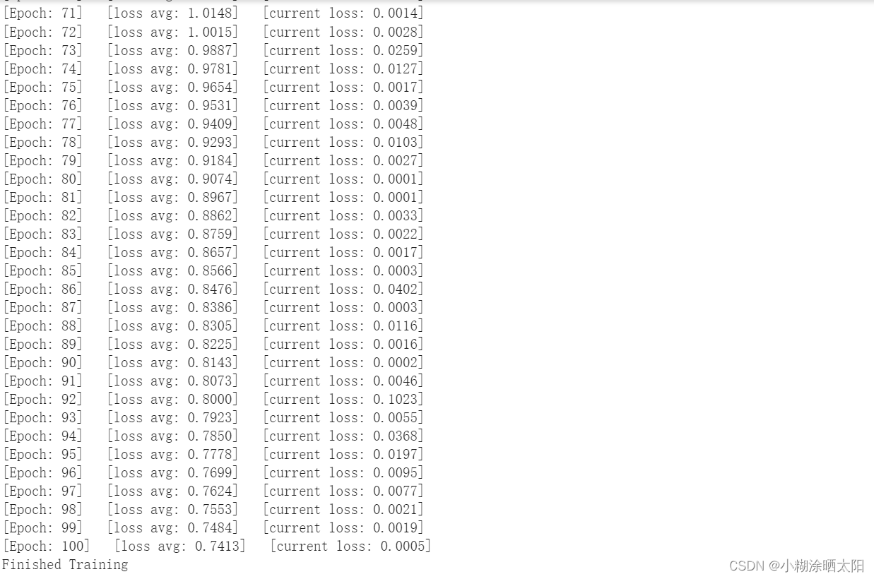
for epoch in range(100):
for i, (inputs, labels) in enumerate(train_loader):
inputs = inputs.to(device)
labels = labels.to(device)
# 优化器梯度归零
optimizer.zero_grad()
# 正向传播 + 反向传播 + 优化
outputs = net(inputs)
loss = criterion(outputs, labels)
loss.backward()
optimizer.step()
total_loss += loss.item()
print('[Epoch: %d] [loss avg: %.4f] [current loss: %.4f]' %(epoch + 1, total_loss/(epoch+1), loss.item()))
print('Finished Training')
#模型测试
count = 0
# 模型测试
for inputs, _ in test_loader:
inputs = inputs.to(device)
outputs = net(inputs)
outputs = np.argmax(outputs.detach().cpu().numpy(), axis=1)
if count == 0:
y_pred_test = outputs
count = 1
else:
y_pred_test = np.concatenate( (y_pred_test, outputs) )
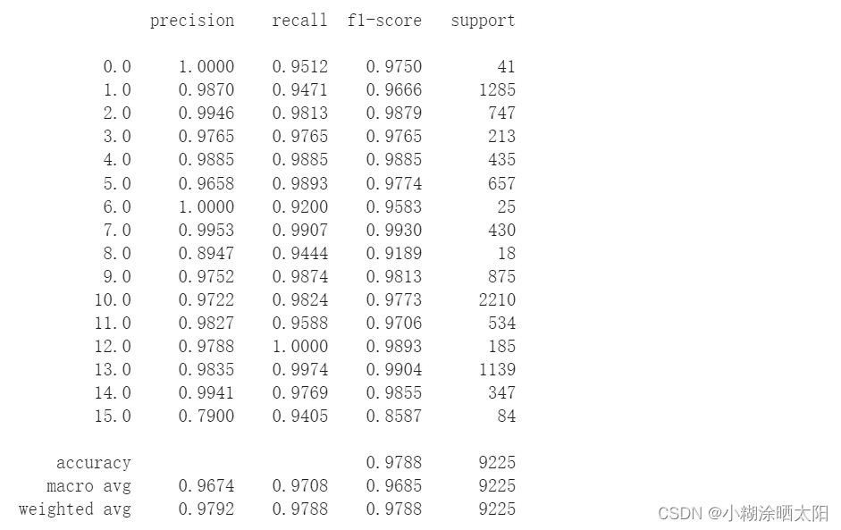
# 生成分类报告
classification = classification_report(ytest, y_pred_test, digits=4)
print(classification)
#备用函数,用于计算各个类准确率
from operator import truediv

def AA_andEachClassAccuracy(confusion_matrix):
    counter = confusion_matrix.shape[0]
    list_diag = np.diag(confusion_matrix)
    list_raw_sum = np.sum(confusion_matrix, axis=1)
    each_acc = np.nan_to_num(truediv(list_diag, list_raw_sum))
    average_acc = np.mean(each_acc)
    return each_acc, average_acc


def reports (test_loader, y_test, name):
    count = 0
    # 模型测试
    for inputs, _ in test_loader:
        inputs = inputs.to(device)
        outputs = net(inputs)
        outputs = np.argmax(outputs.detach().cpu().numpy(), axis=1)
        if count == 0:
            y_pred =  outputs
            count = 1
        else:
            y_pred = np.concatenate( (y_pred, outputs) )

    if name == 'IP':
        target_names = ['Alfalfa', 'Corn-notill', 'Corn-mintill', 'Corn'
                        ,'Grass-pasture', 'Grass-trees', 'Grass-pasture-mowed',
                        'Hay-windrowed', 'Oats', 'Soybean-notill', 'Soybean-mintill',
                        'Soybean-clean', 'Wheat', 'Woods', 'Buildings-Grass-Trees-Drives',
                        'Stone-Steel-Towers']
    elif name == 'SA':
        target_names = ['Brocoli_green_weeds_1','Brocoli_green_weeds_2','Fallow','Fallow_rough_plow','Fallow_smooth',
                        'Stubble','Celery','Grapes_untrained','Soil_vinyard_develop','Corn_senesced_green_weeds',
                        'Lettuce_romaine_4wk','Lettuce_romaine_5wk','Lettuce_romaine_6wk','Lettuce_romaine_7wk',
                        'Vinyard_untrained','Vinyard_vertical_trellis']
    elif name == 'PU':
        target_names = ['Asphalt','Meadows','Gravel','Trees', 'Painted metal sheets','Bare Soil','Bitumen',
                        'Self-Blocking Bricks','Shadows']

    classification = classification_report(y_test, y_pred, target_names=target_names)
    oa = accuracy_score(y_test, y_pred)
    confusion = confusion_matrix(y_test, y_pred)
    each_acc, aa = AA_andEachClassAccuracy(confusion)
    kappa = cohen_kappa_score(y_test, y_pred)

    return classification, confusion, oa*100, each_acc*100, aa*100, kappa*100
classification, confusion, oa, each_acc, aa, kappa = reports(test_loader, ytest, 'IP')
classification = str(classification)
confusion = str(confusion)
file_name = "classification_report.txt"

with open(file_name, 'w') as x_file:
    x_file.write('\n')
    x_file.write('{} Kappa accuracy (%)'.format(kappa))
    x_file.write('\n')
    x_file.write('{} Overall accuracy (%)'.format(oa))
    x_file.write('\n')
    x_file.write('{} Average accuracy (%)'.format(aa))
    x_file.write('\n')
    x_file.write('\n')
    x_file.write('{}'.format(classification))
    x_file.write('\n')
    x_file.write('{}'.format(confusion))
# load the original image
X = sio.loadmat(filepath)['indian_pines_corrected']
y = sio.loadmat(filepath1)['indian_pines_gt']
height = y.shape[0]
width = y.shape[1]
X = applyPCA(X, numComponents= pca_components)
X = padWithZeros(X, patch_size//2)
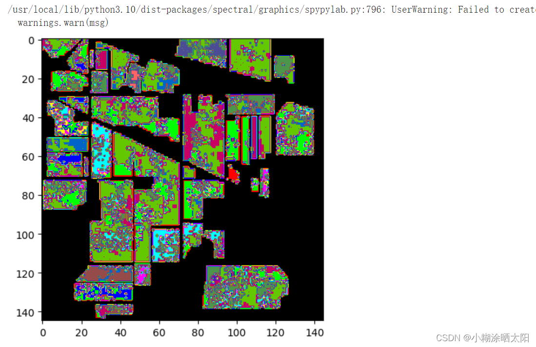
# 逐像素预测类别
outputs = np.zeros((height,width))
for i in range(height):
for j in range(width):
if int(y[i,j]) == 0:
continue
else :
image_patch = X[i:i+patch_size, j:j+patch_size, :]
image_patch = image_patch.reshape(1,image_patch.shape[0],image_patch.shape[1], image_patch.shape[2], 1)
X_test_image = torch.FloatTensor(image_patch.transpose(0, 4, 3, 1, 2)).to(device)
prediction = net(X_test_image)
prediction = np.argmax(prediction.detach().cpu().numpy(), axis=1)
outputs[i][j] = prediction+1
if i % 20 == 0:
print('... ... row ', i, ' handling ... ...')
predict_image = spectral.imshow(classes = outputs.astype(int),figsize =(5,5))
● 训练HybridSN,然后多测试几次,会发现每次分类的结果都不一样,请思考为什么?
在进行训练时会采用梯度下降的方法,这些方法可能会找到局部最优解,但是因为你的学习率也就是你的步长设置的不够大,
就会导致模型被困在局部最优解,无法跳出。 其次,你每次训练的时候,神经网络的参数和权重每次都是随机的,所以肯定每次的结果都不一样。
● 如果想要进一步提升高光谱图像的分类性能,可以如何改进?
扫描二维码关注公众号,回复:
16308401 查看本文章

1.增加大量、可靠的训练样本,提高泛化性能。
2.选择合适的网络结构。
3.确定超参数:在训练过程中,检验模型的状态、收敛情况。通常用来调整超参数,通过几组模型在验证集上的表现确定超参数。
4.对特征图每个位置进行二维调整(即attention调整),使模型关注到值得更多关注的区域上。
● depth-wise conv 和 分组卷积有什么区别与联系?
分组卷积只进行一次卷积操作即可,而深度可分离卷积需要进行两次——先depth_wise再point_wise卷积,但他们本质上是一样的。
深度可分离卷积进行一次卷积是无法达到输出指定维度的tensor的,这是由它将group设为in_channel决定的,输出的tensor通道数只能是in_channel,不能达到要求,
所以又用了1*1的卷积改变最终输出的通道数。这样的想法也是自然而然的,BottleNeck不就是先1*1卷积减少参数量再3*3卷积feature map,最后再1*1恢复原来的通道数,
所以BottleNeck的目的就是减少参数量。提到BottleNeck结构就是想说明1*1卷积经常用来改变通道数。
● SENet 的注意力是不是可以加在空间位置上?
● 在 ShuffleNet 中,通道的 shuffle 如何用代码实现?
def channel_shuffle(x: Tensor, groups: int) -> Tensor:

    batch_size, num_channels, height, width = x.size()
    channels_per_group = num_channels // groups

    # reshape
    # [batch_size, num_channels, height, width] -> [batch_size, groups, channels_per_group, height, width]
    x = x.view(batch_size, groups, channels_per_group, height, width)

    x = torch.transpose(x, 1, 2).contiguous()

    # flatten
    x = x.view(batch_size, -1, height, width)

    return x