Python非线性回归

非线性样本

from matplotlib import pyplot as mp
y = [.4187, .0964, .0853, .0305, .0358, .0338, .0368, .0222, .0798, .1515]
x = [[i]for i in range(len(y))]
mp.scatter(x, y, s=99)
mp.show()

Sklearn回归汇总

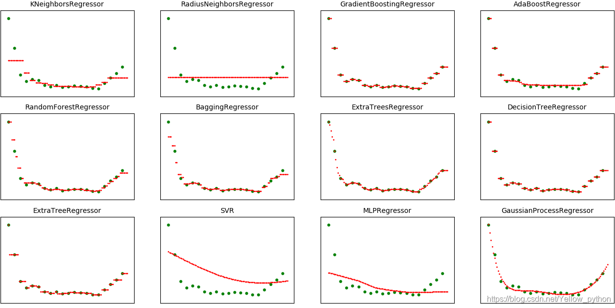
import matplotlib.pyplot as mp
# 训练集
y = [.27, .16, .06, .036, .044, .04, .022, .017, .022, .014, .017, .02, .019, .017, .011, .01, .03, .05, .066, .09]
ly, n = len(y), 100
x = [[i / ly]for i in range(ly)]
# 待测集
w = [[i / n] for i in range(n)]
# # x轴范围
# max_x = 1
# x, w = [[i[0]*max_x] for i in x], [[i[0]*max_x] for i in w]

def modeling(models):
    for i in range(len(models)):
        print(models[i].__name__)
        # 建模、拟合
        model = models[i]()
        model.fit(x, y)
        # 预测
        z = model.predict(w)
        # 可视化
        mp.subplot(3, 4, i + 1)
        mp.title(models[i].__name__, size=10)
        mp.xticks(())
        mp.yticks(())
        mp.scatter(x, y, s=11, color='g')
        mp.scatter(w, z, s=1, color='r')
    mp.show()

from sklearn.neighbors import KNeighborsRegressor, RadiusNeighborsRegressor
from sklearn.ensemble import GradientBoostingRegressor, AdaBoostRegressor,\
    RandomForestRegressor, BaggingRegressor, ExtraTreesRegressor, VotingRegressor
from sklearn.tree import DecisionTreeRegressor, ExtraTreeRegressor
from sklearn.svm import SVR
from sklearn.neural_network import MLPRegressor
from sklearn.gaussian_process import GaussianProcessRegressor
modeling([
    KNeighborsRegressor, RadiusNeighborsRegressor,
    GradientBoostingRegressor, AdaBoostRegressor, RandomForestRegressor, BaggingRegressor, ExtraTreesRegressor,
    # VotingRegressor,
    DecisionTreeRegressor, ExtraTreeRegressor,
    SVR, MLPRegressor, GaussianProcessRegressor
])

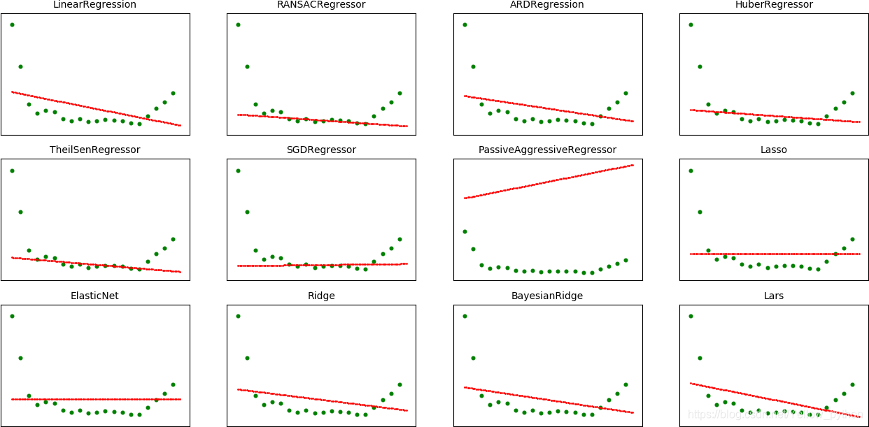
from sklearn.linear_model import LinearRegression, RANSACRegressor, ARDRegression, HuberRegressor, TheilSenRegressor,\
    SGDRegressor, PassiveAggressiveRegressor, Lasso, ElasticNet, Ridge, BayesianRidge, Lars
modeling([
    LinearRegression, RANSACRegressor, ARDRegression, HuberRegressor, TheilSenRegressor,
    SGDRegressor, PassiveAggressiveRegressor, Lasso, ElasticNet, Ridge, BayesianRidge, Lars
])

决策树

import matplotlib.pyplot as mp
# 训练集
y = [.4187, .0964, .0853, .0305, .0358, .0338, .0368, .0222, .0798, .1515]
x = [[i]for i in range(len(y))]
# 待测集
w = [[i / 100 * len(y)] for i in range(100)]

def modeling(models):
    n = len(models)
    for i in range(n):
        # 建模、拟合
        models[i].fit(x, y)
        # 预测
        z = models[i].predict(w)
        # 可视化
        mp.subplot(1, n, i + 1)
        mp.scatter(x, y, s=22, color='g')
        mp.scatter(w, z, s=2, color='r')
    mp.show()

from sklearn.tree import DecisionTreeRegressor
modeling([
    DecisionTreeRegressor(max_depth=1),
    DecisionTreeRegressor(max_depth=2),
    DecisionTreeRegressor(max_depth=3),
    DecisionTreeRegressor(max_depth=4),
    DecisionTreeRegressor(),
])

随机森林

import matplotlib.pyplot as mp
# 训练集
y = [.4187, .0964, .0853, .0305, .0358, .0338, .0368, .0222, .0798, .1515]
x = [[i]for i in range(len(y))]
# 待测集
w = [[i / 100 * len(y)] for i in range(100)]

def modeling(models):
    n = len(models)
    for i in range(n):
        # 建模、拟合
        models[i].fit(x, y)
        # 预测
        z = models[i].predict(w)
        # 可视化
        mp.subplot(1, n, i + 1)
        mp.scatter(x, y, s=22, color='g')
        mp.scatter(w, z, s=2, color='r')
    mp.show()

from sklearn.ensemble import RandomForestRegressor
modeling([
    RandomForestRegressor(max_depth=1),
    RandomForestRegressor(max_depth=2),
    RandomForestRegressor(),
])

高斯过程

高斯过程回归：使用高斯过程先验对数据进行回归分析的非参数模型（non-parameteric model）
算法特征：计算开销大，通常用于低维和小样本的回归问题
应用领域：时间序列分析、图像处理和自动控制等

from sklearn.gaussian_process import GaussianProcessRegressor
import matplotlib.pyplot as mp, random
# 创建样本
a = [199, 188, 170, 157, 118, 99, 69, 44, 22, 1, 5, 9, 15, 21, 30, 40, 50, 60, 70, 79, 88, 97, 99, 98, 70, 46, 39, 33]
for e, y in enumerate((a, [a[i//2]+random.randint(0, 30) for i in range(len(a)*2)])):
    # 待测集
    ly, n = len(y), 2000
    w = [[i / n * 1.2 - .1] for i in range(n)]
    # 建模、拟合、预测
    model = GaussianProcessRegressor()
    model.fit([[i/ly]for i in range(ly)], y)
    z = model.predict(w)
    # 可视化
    mp.subplot(1, 2, e + 1)
    mp.yticks(())
    mp.bar([i/ly for i in range(ly)], y, width=.7/ly)
    mp.scatter(w, z, s=1, color='r')
mp.show()

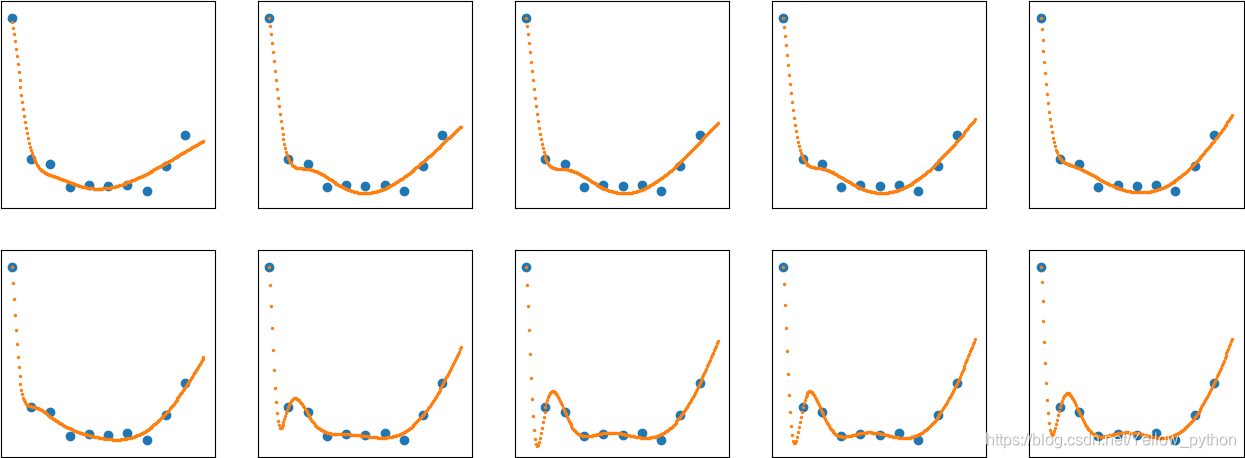
Keras神经网络

from matplotlib import pyplot
from keras.models import Sequential
from keras.layers import Dense
from keras.optimizers import Adam

# 训练集
y = [.27, .16, .06, .036, .044, .04, .022, .017, .022, .014, .017, .02, .019, .017, .011, .01, .03, .05, .066, .09]
x = list(range(len(y)))
# 待测集
n = 200
w = [i/n*len(y) for i in range(n)]

# 建模
model = Sequential()
model.add(Dense(units=10, input_dim=1, activation='sigmoid'))
model.add(Dense(units=1, activation='sigmoid'))
# 编译、优化
model.compile(optimizer=Adam(), loss='mse')

for i in range(10):
    # 训练
    model.fit(x, y, epochs=2500, verbose=0)
    print(i, 'loss', model.evaluate(x, y, verbose=0))
    # 预测
    z = model.predict(w)
    # 可视化
    pyplot.subplot(2, 5, i + 1)
    pyplot.xticks(())
    pyplot.yticks(())
    pyplot.scatter(x, y)  # 样本点
    pyplot.scatter(w, z, s=2)  # 预测线
pyplot.show()